[the sixth operation of modern signal processing]

1. The definition of circular convolution is as follows

The defined length is N The finite length sequence of Cyclic convolution of （ Circular convolution ）
$$x_1(n)\otimes x_2(n)=\sum _{i=0}^{N-1}{x}_1(i)x_2((n-i){)}_N$$
The length of the sequence obtained by cyclic convolution is still N, The length remains the same .
among Said to Move the circle to the right m operation , If the length is 6 Sequence , The figure and the figure of circular displacement are shown in the following figure ：

（a） （b） （c）
The length is N Sequence Through the length of L（ L<N） The system of , The response can be defined by circular convolution as
$$y(n)=x_1(n)\otimes h_1(n)=\sum _{i=0}^{N-1}{x}_1(i)h_1((n-i){)}_N$$
among Yes, it will The length of extends to N（ Zero compensation ） obtain .
If the length is 4 The finite length sequence of x(n)={1,1,1,1}, Through the system h(n)={n=0,1,2}, Then there are $$h_1(n)=1,2,0,0$$ The response is a
$$y(0)=x(0)h_1((0){)}_4+x_1(1)h_1((-1){)}_4+x_1(2)h_1((-2){)}_4+x(3)h_1((-3){)}_3$$
$$=x_1(0)h_1(0)+x_1(1)h_1(3)+x_1(2)h_1(2)+x(3)h_1(1)$$
$$y(1)=x(0)h_1((1){)}_4+x_1(1)h_1((0){)}_4+x_1(2)h_1((-1){)}_4+x(3)h_1((-2){)}_3$$
$$=x_1(0)h_1(1)+x_1(1)h_1(0)+x_1(2)h_1(3)+x(3)h_1(2).....$$
Refer to the convolution algorithm we talked about in class to complete the following problems
problem ： Sequence $$x(n)=cos(0.2\pi n)$$, Through the system $$h_1(n)=1,2,0,0$$ ;
（1） use matlab Complete the results of the following circular convolution （ The length of is taken as 100）, And with matlab Of cconv(x1,x2,N) Function results are compared .
（2） Compare circular convolution with linear convolution （conv Ordinary convolution ） The result obtained , Analyze the advantages of circular convolution .（20 branch ）
Explain ：（1）
Code ：
Define the circular convolution function circonvt

function y=circonvt(x1,x2,N) 
x_1=[x1 zeros(1,N-length(x1))]; 
h_1=[x2 zeros(1,N-length(x2))]; 
y1=conv(x_1,h_1);
z_1=[zeros(1,N) y1(1:(N-1))]; 
z_2=[y1((N+1):(2*N-1)) zeros(1,N)];
z=z_1(1:(2*N-1))+z_2(1:(2*N-1))+y1(1:(2*N-1)); 
y=z(10:N+10);
end

%% 1 The definition of circular convolution is as follows 
%（1）
clc;clear;
n=20;
t=0:99;
t1=0:n-1;
xn=cos(0.2*pi*t);
hn=[1,-2,2,-1,zeros(1,96)];
y1=circonvt(xn,hn,100);
y2=cconv(xn,hn,100);
hn=hn(1:n);
Y1=y1(1:n);
Y2=y2(1:n);
figure(1);
subplot(1,3,1);
stem(t,xn); ylabel ('hn'); xlabel ('t');title('xn The original signal '); grid on;
subplot(1,3,2);
stem(t1,Y1); ylabel ('Y1'); xlabel ('t');title(' Custom circular convolution circonvt'); grid on;
subplot(1,3,3);
stem(t1,Y2); ylabel ('Y2'); xlabel ('t');title('matlab Circular convolution cconv'); grid on;
hold on;
%%

Pictured 1：

chart 1
It can be seen from the above figure , The two images are consistent , It indicates that the function structure is correct .
（2）
Code ：

%（2）
y3=conv(xn,hn);
Y3=y3(1:n);
figure(2);
subplot(1,3,1);
stem(t,xn); ylabel ('hn'); xlabel ('t');title('xn The original signal '); grid on;
subplot(1,3,2);
stem(t1,Y2); ylabel ('Y2'); xlabel ('t');title('matlab Circular convolution cconv'); grid on;
subplot(1,3,3);
stem(t1,Y3); ylabel ('Y3'); xlabel ('t');title('matlab linear convolution conv'); grid on;
%%

Pictured 2：

chart 2
Comparative analysis shows that , Circular convolution is a periodic function , Linear convolution is not a periodic function , The period after linear convolution is consistent with circular convolution .

2. DTFT and DFT Transformation

Infinite sequence ,（1） Draw the amplitude spectrum ;（2） Cut the length of the sequence N=128 The finite length sequence of , Draw a picture of it DTFT Spectrum and DFT spectrum .（3） The steps and methods of analyzing signal spectrum by means of Fourier transform are illustrated , And point out that it will bring about those distortions ？（20 branch ）
Explain ：（1）
Code ：
dfs function

function[Xk]=dfs(xn,N)
n=0:N-1;
k=0:N-1;
WN=exp(-j*2*pi/N);
nk=n'*k;
Xk=(xn*WN.^nk)/N;
end

Idfs function

function[xn]=Idfs(Xk,N)
n=0:N-1;
k=0:N-1;
WN=exp(j*2*pi/N);
nk=n'*k;
xn=(Xk*WN.^nk);
end

%% 2
% (1)
clc;clear;
n=0:0.01:2*pi;
x1n=(0.98).^n;
N = size(n,2);
Xk = dfs(x1n, N);
figure(3);
plot(n,abs(Xk));ylabel ('|Xk|'); xlabel ('n'); title(' The amplitude spectrum of the original sequence '); % Display the amplitude spectrum of the sequence 
hold on;
%%

Pictured 3：

chart 3

（2）
Code ：

%%
% (2)
n2 = 0:128;
n2 = n2*2*pi/128;
x128n=(0.98).^n2;
N2 = size(x128n,2);
X128k = dfs(x128n,N2);
k128 = 0:N2-1;
figure(4);
subplot(1,2,1);%2*2 The first in the graph 
plot(k128,abs(X128k)); ylabel ('|X128k|'); xlabel ('k128');  title('128 Sequential DTFT spectrum ');
subplot(1,2,2);
stem(k128,abs(X128k)); ylabel ('|X128k|'); xlabel ('k128'); title('128 Sequential DFT spectrum ');
hold on;
%%

Pictured 4：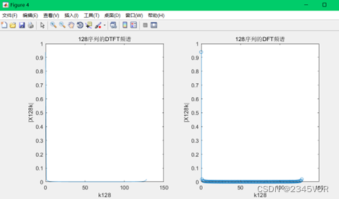

chart 4
(3)
The steps of Fourier transform to analyze signal spectrum ： First discrete and then Fourier transform
Method ：dfs /fft
From the figure 4 You know , Infinite sequence after interception , Its spectrum will be distorted , This distortion is called interception distortion . The smaller the intercept length, the more serious the distortion . After truncating an infinite sequence , Its spectrum will produce distortion , This distortion is called interception distortion .

3. Wavelet forced denoising

Construct a sinusoidal signal + noise , Use only matlab Of dwt(x,’wname’) and idwt(ca1,cd1,‘db2’) Function to complete the simulation of wavelet forced de-noising . among wname We adopt db1 and db2、 Wavelet denoising adopts primary decomposition and secondary decomposition , in total 4 Simulation results , Analyze the signal-to-noise ratio before and after denoising .（20 branch ）
Explain ：
Code ：

%% 3
clc;clear
X = 10*sin(0:pi/100:6*pi);
Y = awgn(X,15,'measured');
sigPower = sum(abs(X).^2)/length(X)           % Calculate the signal power 
noisePower=sum(abs(Y-X).^2)/length(Y-X)  % Calculate the noise power 
SNR=10*log10(sigPower/noisePower)          % Calculate the signal-to-noise ratio from the definition of signal-to-noise ratio , Unit is db
figure(5);
subplot(5,1,1);plot(Y);
xlabel(' Sampling point '); ylabel(' The amplitude ');title(sprintf(' The original signal , Signal-to-noise ratio  %f',SNR));
% db1 Break it down for the first time 
[ca1,cd1]=dwt(Y,'db1');
cd1=zeros(1,length(cd1));
X1=idwt(ca1,cd1,'db1');
X1=X1(1,1:601);
sigPower = sum(abs(X1).^2)/length(X1)           % Calculate the signal power 
noisePower=sum(abs(X1-X).^2)/length(X1-X)  % Calculate the noise power 
SNR=10*log10(sigPower/noisePower)          % Calculate the signal-to-noise ratio from the definition of signal-to-noise ratio , Unit is db
subplot(5,1,2);plot(X1);
xlabel(' Sampling point '); ylabel(' The amplitude ');title(sprintf('db1 Break it down for the first time , Signal-to-noise ratio  %f',SNR));
% db1 The second decomposition 
[ca2,cd2]=dwt(X1,'db1');
cd2=zeros(1,length(cd2));
X2=idwt(ca2,cd2,'db1');
X2=X2(1,1:601);
sigPower = sum(abs(X2).^2)/length(X2)           % Calculate the signal power 
noisePower=sum(abs(X2-X).^2)/length(X2-X)  % Calculate the noise power 
SNR2=10*log10(sigPower/noisePower)          % Calculate the signal-to-noise ratio from the definition of signal-to-noise ratio , Unit is db
subplot(5,1,3);plot(X2);
xlabel(' Sampling point '); ylabel(' The amplitude ');title(sprintf('db1 The second decomposition , Signal-to-noise ratio  %f',SNR2));
% db2 Break it down for the first time 
[ca3,cd3]=dwt(Y,'db2');
cd3=zeros(1,length(cd3));
X3=idwt(ca3,cd3,'db2');
X3=X3(1,1:601);
sigPower = sum(abs(X3).^2)/length(X3)           % Calculate the signal power 
noisePower=sum(abs(X3-X).^2)/length(X3-X)  % Calculate the noise power 
SNR3=10*log10(sigPower/noisePower)          % Calculate the signal-to-noise ratio from the definition of signal-to-noise ratio , Unit is db
subplot(5,1,4);plot(X3);
xlabel(' Sampling point '); ylabel(' The amplitude ');title(sprintf('db2 Break it down for the first time , Signal-to-noise ratio  %f',SNR3));
% db2 The second decomposition 
[ca4,cd4]=dwt(X3,'db2');
cd4=zeros(1,length(cd4));
X4=idwt(ca4,cd4,'db2');
X4=X4(1,1:601);
sigPower = sum(abs(X4).^2)/length(X4)           % Calculate the signal power 
noisePower=sum(abs(X4-X).^2)/length(X4-X)  % Calculate the noise power 
SNR4=10*log10(sigPower/noisePower)          % Calculate the signal-to-noise ratio from the definition of signal-to-noise ratio , Unit is db
subplot(5,1,5);plot(X4);
xlabel(' Sampling point '); ylabel(' The amplitude ');title(sprintf('db2 The second decomposition , Signal-to-noise ratio  %f',SNR4));

Pictured 5：

chart 5
We can see by comparing the images before and after , For this model, the signal-to-noise ratio has been significantly improved ,db1 Than db2 Forced noise removal is obvious .

4. Quadratic wavelet image transform

Using quadratic wavelet transform function dwt2 Complete a picture 2 Subwavelet transform , And use idwt2 Realization 2 Image restoration after sub wavelet decomposition .（20 branch ）
Explain ：
Code ：

%% 
% idwt2 function 
%  function ： Two dimensional discrete wavelet inverse transform 
clc;clear;
load woman;
nbcol = size(map,1);% Returns the number of rows and columns of the matrix 
[cA1,cH1,cV1,cD1]=dwt2(X,'db1');
cod_x=wcodemat(X,nbcol);% Return matrix X The coding matrix of ,nbcol Is the maximum value of the encoding 
cod_cA1=wcodemat(cA1,nbcol);
cod_cH1=wcodemat(cH1,nbcol);
cod_cV1=wcodemat(cV1,nbcol);
cod_cD1=wcodemat(cD1,nbcol);
dec2d=[cod_cA1,cod_cH1;cod_cV1,cod_cD1];
A0=idwt2(cA1,cH1,cV1,cD1,'db1');
figure(10);
subplot(2,2,1),imshow(X,[]);
title(' original image ');
subplot(2,2,2),imshow(dec2d,[])
title(' Two dimensional discrete wavelet decomposition of the image ');
subplot(2,2,3),imshow(X,[])
title(' original image ');
subplot(2,2,4),imshow(A0,[])
title(' The image reconstructed by two-dimensional wavelet decomposition ');
%%

Pictured 6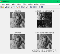

chart 6
test Complete code ：

%% 1 The definition of circular convolution is as follows 
%（1）
clc;clear;
n=20;
t=0:99;
t1=0:n-1;
xn=cos(0.2*pi*t);
hn=[1,-2,2,-1,zeros(1,96)];
y1=circonvt(xn,hn,100);
y2=cconv(xn,hn,100);
hn=hn(1:n);
Y1=y1(1:n);
Y2=y2(1:n);
figure(1);
subplot(1,3,1);
stem(t,xn); ylabel ('hn'); xlabel ('t');title('xn The original signal '); grid on;
subplot(1,3,2);
stem(t1,Y1); ylabel ('Y1'); xlabel ('t');title(' Custom circular convolution circonvt'); grid on;
subplot(1,3,3);
stem(t1,Y2); ylabel ('Y2'); xlabel ('t');title('matlab Circular convolution cconv'); grid on;
hold on;
%(2)
y3=conv(xn,hn);
Y3=y3(1:n);
figure(2);
subplot(1,3,1);
stem(t,xn); ylabel ('hn'); xlabel ('t');title('xn The original signal '); grid on;
subplot(1,3,2);
stem(t1,Y2); ylabel ('Y2'); xlabel ('t');title('matlab Circular convolution cconv'); grid on;
subplot(1,3,3);
stem(t1,Y3); ylabel ('Y3'); xlabel ('t');title('matlab linear convolution conv'); grid on;

%% 2
% (1)
clc;clear;
n=0:0.01:2*pi;
x1n=(0.98).^n;
N = size(n,2);
Xk = dfs(x1n, N);
figure(3);
plot(n,abs(Xk));ylabel ('|Xk|'); xlabel ('n'); title(' The amplitude spectrum of the original sequence '); % Display the amplitude spectrum of the sequence 
hold on;
% (2)
n2 = 0:128;
n2 = n2*2*pi/128;
x128n=(0.98).^n2;
N2 = size(x128n,2);
X128k = dfs(x128n,N2);
k128 = 0:N2-1;
figure(4);
subplot(1,2,1);%2*2 The first in the graph 
plot(k128,abs(X128k)); ylabel ('|X128k|'); xlabel ('k128');  title('128 Sequential DTFT spectrum ');
subplot(1,2,2);
stem(k128,abs(X128k)); ylabel ('|X128k|'); xlabel ('k128'); title('128 Sequential DFT spectrum ');
hold on;


%% 3
clc;clear
X = 10*sin(0:pi/100:6*pi);
Y = awgn(X,15,'measured');
sigPower = sum(abs(X).^2)/length(X)           % Calculate the signal power 
noisePower=sum(abs(Y-X).^2)/length(Y-X)  % Calculate the noise power 
SNR=10*log10(sigPower/noisePower)          % Calculate the signal-to-noise ratio from the definition of signal-to-noise ratio , Unit is db
figure(5);
subplot(5,1,1);plot(Y);
xlabel(' Sampling point '); ylabel(' The amplitude ');title(sprintf(' The original signal , Signal-to-noise ratio  %f',SNR));
% db1 Break it down for the first time 
[ca1,cd1]=dwt(Y,'db1');
cd1=zeros(1,length(cd1));
X1=idwt(ca1,cd1,'db1');
X1=X1(1,1:601);
sigPower = sum(abs(X1).^2)/length(X1)           % Calculate the signal power 
noisePower=sum(abs(X1-X).^2)/length(X1-X)  % Calculate the noise power 
SNR=10*log10(sigPower/noisePower)          % Calculate the signal-to-noise ratio from the definition of signal-to-noise ratio , Unit is db
subplot(5,1,2);plot(X1);
xlabel(' Sampling point '); ylabel(' The amplitude ');title(sprintf('db1 Break it down for the first time , Signal-to-noise ratio  %f',SNR));
% db1 The second decomposition 
[ca2,cd2]=dwt(X1,'db1');
cd2=zeros(1,length(cd2));
X2=idwt(ca2,cd2,'db1');
X2=X2(1,1:601);
sigPower = sum(abs(X2).^2)/length(X2)           % Calculate the signal power 
noisePower=sum(abs(X2-X).^2)/length(X2-X)  % Calculate the noise power 
SNR2=10*log10(sigPower/noisePower)          % Calculate the signal-to-noise ratio from the definition of signal-to-noise ratio , Unit is db
subplot(5,1,3);plot(X2);
xlabel(' Sampling point '); ylabel(' The amplitude ');title(sprintf('db1 The second decomposition , Signal-to-noise ratio  %f',SNR2));
% db2 Break it down for the first time 
[ca3,cd3]=dwt(Y,'db2');
cd3=zeros(1,length(cd3));
X3=idwt(ca3,cd3,'db2');
X3=X3(1,1:601);
sigPower = sum(abs(X3).^2)/length(X3)           % Calculate the signal power 
noisePower=sum(abs(X3-X).^2)/length(X3-X)  % Calculate the noise power 
SNR3=10*log10(sigPower/noisePower)          % Calculate the signal-to-noise ratio from the definition of signal-to-noise ratio , Unit is db
subplot(5,1,4);plot(X3);
xlabel(' Sampling point '); ylabel(' The amplitude ');title(sprintf('db2 Break it down for the first time , Signal-to-noise ratio  %f',SNR3));
% db2 The second decomposition 
[ca4,cd4]=dwt(X3,'db2');
cd4=zeros(1,length(cd4));
X4=idwt(ca4,cd4,'db2');
X4=X4(1,1:601);
sigPower = sum(abs(X4).^2)/length(X4)           % Calculate the signal power 
noisePower=sum(abs(X4-X).^2)/length(X4-X)  % Calculate the noise power 
SNR4=10*log10(sigPower/noisePower)          % Calculate the signal-to-noise ratio from the definition of signal-to-noise ratio , Unit is db
subplot(5,1,5);plot(X4);
xlabel(' Sampling point '); ylabel(' The amplitude ');title(sprintf('db2 The second decomposition , Signal-to-noise ratio  %f',SNR4));
%% 4  Quadratic wavelet transform function dwt2
% idwt2 function 
%  function ： Two dimensional discrete wavelet inverse transform 
clc;clear;
load woman;
nbcol = size(map,1);% Returns the number of rows and columns of the matrix 
[cA1,cH1,cV1,cD1]=dwt2(X,'db1');
cod_x=wcodemat(X,nbcol);% Return matrix X The coding matrix of ,nbcol Is the maximum value of the encoding 
cod_cA1=wcodemat(cA1,nbcol);
cod_cH1=wcodemat(cH1,nbcol);
cod_cV1=wcodemat(cV1,nbcol);
cod_cD1=wcodemat(cD1,nbcol);
dec2d=[cod_cA1,cod_cH1;cod_cV1,cod_cD1];
A0=idwt2(cA1,cH1,cV1,cD1,'db1');
figure(6);
subplot(2,2,1),imshow(X,[]);
title(' original image ');
subplot(2,2,2),imshow(dec2d,[])
title(' Two dimensional discrete wavelet decomposition of the image ');
subplot(2,2,3),imshow(X,[])
title(' original image ');
subplot(2,2,4),imshow(A0,[])
title(' The image reconstructed by two-dimensional wavelet decomposition ');

5. Experience and experience

Share the experience of learning this course ; And connected with their own research direction , How to apply the learned knowledge to future scientific research （1000 Word left or right ）.

Learning experience of modern signal processing
First of all, thank you very much for your passionate speech in the past eight weeks , Let us deeply appreciate the charm of modern signal processing , No matter where we come from , How about major , The teacher explained to us bit by bit from the most basic , Very rare and valuable ！
Looking back at the eight weeks of systematic learning , Deeply feel the teacher's mathematical literacy , Solid foundation , It is worth following and learning . Start with the signal sampling , We know that our world is basically a finite discretization of infinite sequences , Then we can find out the rules and characteristics , To capture the most subtle essence . Then we explore the essence of convolution , The code taught us how to understand his thoughts and the mathematical principles behind it bit by bit . Although there are many episodes in this process , But the teacher still overcame all difficulties . Like we showed the mystery .
Random digital signal processing is formed by the interdisciplinary knowledge , In communication 、 radar 、 Voice Processing 、 Image processing 、 acoustics 、 Seismology 、 geological prospecting 、 Meteorology 、 remote sensing 、 Biomedical engineering 、 Nuclear Engineering 、 Space engineering and other fields are inseparable from random digital signal processing . With the progress of computer technology , Random digital signal processing technology has developed rapidly . This course mainly studies two main problems of random digital signal processing : Filter design and spectrum analysis . In digital signal processing , Filtering technology occupies an extremely important position . Digital filtering is speech and image processing 、 pattern recognition 、 A basic processing algorithm in applications such as spectrum analysis . But in many applications , Often have to deal with some unpredictable signals 、 Noise or time-varying signal , If the digital filter with fixed filtering coefficient is used, the optimal filtering cannot be realized . under these circumstances , Adaptive filter must be designed , So that the dynamic characteristic of the filter changes with the change of signal and noise , To achieve the optimal filtering effect .
Also learned the wavelet transform. This paper introduces the use of wavelet to complete ： Discontinuity identification 、 Time frequency analysis ( The short-time Fourier transform )、 Signal denoising . Some useful conclusions obtained in this paper are listed below ： High frequency detail coefficient image in wavelet domain , It is specially used to check the discontinuity of the original signal ; As the number of decomposition increases , The coefficient image of the most advanced high-frequency detail almost only reflects the position of the discontinuity ！ The purpose of time-frequency analysis is to observe the transformation law of if rate of original signal with time , Window size is a key parameter ; In reality, time-frequency diagrams are basically connected ; Wavelet denoising uses many functions , And it is often used together .
I think the next study can be related to my major , The direction that has been basically determined is 3D Printer fault diagnosis , This is because visual information is not only used for fault diagnosis , In addition, it will be added to the sound vibration for load diagnosis , So wavelet transform is very useful 3D Printer fault diagnosis is temporarily divided into four categories , One is broken wire , Then the second one is laminar , The third is that there is wire drawing , The fourth model is off the platform , As for the big picture , Visual convolution neural network can be used to distinguish , Sound sensors can be used for both written and wire drawing , Make a fine division . Thank you again for your teachers and classmates ！！！