当前位置:网站首页>Machine learning 3.2 decision tree model learning notes (to be supplemented)
Machine learning 3.2 decision tree model learning notes (to be supplemented)
2022-07-03 11:27:00 【HeartFireY】
3.2.1 Model structure
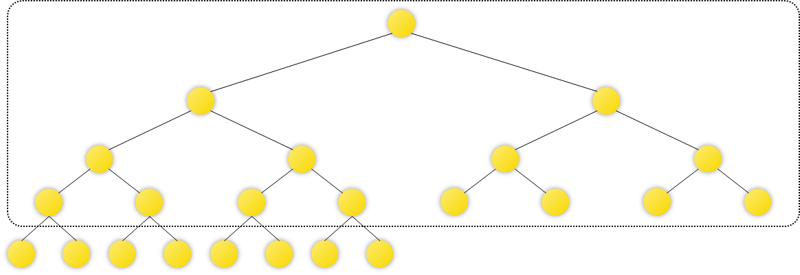
The decision tree model abstracts the thinking process into a series of discrimination and decision-making processes of known data attributes , Use tree structure to express the logic and relationship of discrimination and a series of discrimination processes , The results of discrimination or decision-making are expressed by leaf nodes .

As shown in the figure above , All leaf nodes on a tree represent the final result , Instead of leaf nodes, they represent the points of each decision , That is, the discrimination of a certain attribute of the sample . It is not difficult to find that the decision tree is an extrovert tree model , Each internal node will directly or indirectly affect the final result of the decision . The path from the root node to a leaf node is called the test sequence .
We can describe the construction process of decision tree model as the following process :
- According to some classification rules, the optimal classification features are obtained , Calculate the optimal eigenfunction , And create the partition node of the feature , The data set is divided into Ruo cadre molecular data set according to the division node ;
- Reuse discriminant rules in sub datasets , Construct a new node , As a new branch of the tree ;
- When generating sub datasets , Pay attention to check whether the data belong to the same category or have no attributes for data division anymore ; If you can still continue to classify , Then recursively execute the above process ; Otherwise, take the current node as the leaf node , End the construction of this branch .
3.2.2 Criteria
The key of constructing decision tree is to reasonably select the sample attributes corresponding to its temporal nodes , Make the samples in the sample book subset corresponding to the node belong to the same category as much as possible , That is, it has the highest purity possible .
The criteria of decision tree model need to meet the following two points :
- If the samples in the corresponding data subset of the node basically belong to the same category , There is no need to further divide the data subset of the node , Otherwise, it is necessary to further divide the data subset of the node , Generate new criteria ;
- If the new criterion can basically separate different types of data on the node , So that each child node is data with a single category , Then the criterion is a good rule , Otherwise, it is necessary to re select the criteria .
How to quantify the selection criteria of discriminant attributes of decision tree ?
We generally use information entropy ( entropy ) Quantitative analysis of the purity of the sample set . Information entropy is a kind of measurement index that quantitatively describes the uncertainty of random variables in information theory , It is mainly used to measure the disorder degree of data value , The larger the entropy value, the more disorderly the data value is .
hypothesis ξ \xi ξ For having n n n Possible values { s 1 , s 2 , … , s n } \{s_1, s_2, \dots, s_n\} { s1,s2,…,sn} Discrete random variable , The probability distribution is P ( ξ = s i ) = p i P(\xi = s_i) = p_i P(ξ=si)=pi, Then its information entropy is defined as :
H ( ξ ) = − ∑ i = 1 n p i log 2 p i H(\xi) = - \sum^{n}_{i = 1}p_i\log_2p_i H(ξ)=−i=1∑npilog2pi
When H ( ξ ) H(\xi) H(ξ) The larger the value of , Indicates a random variable ξ \xi ξ The greater the uncertainty .
For any given two discrete random variables ξ , η \xi, \eta ξ,η, Its joint probability distribution is :
P ( ξ = s i , η = t i ) = p i j , i = 1 , 2 , … , n ; j = 1 , 2 , … , m P(\xi = s_i, \eta = t_i) = p_{ij}, i = 1, 2, \dots, n; j = 1, 2, \dots, m P(ξ=si,η=ti)=pij,i=1,2,…,n;j=1,2,…,m
be η \eta η About ξ \xi ξ The entropy of information H ( η ∣ ξ ) H(\eta\ | \ \xi) H(η ∣ ξ) Quantitative representation in known random variables ξ \xi ξ Random variable under the condition of value η \eta η Uncertainty of value , The calculation formula is random variable η \eta η Entropy of random variables based on conditional probability distribution ξ \xi ξ Mathematical expectation , That is to say :
H ( η ∣ ξ ) = ∑ i = 1 n p i H ( η ∣ ξ = s i ) H(\eta\ | \ \xi) = \sum^{n}_{i = 1}{p_iH(\eta\ | \ \xi = s_i)} H(η ∣ ξ)=i=1∑npiH(η ∣ ξ=si)
among , p i = P ( ξ = s i ) , i = 1 , 2 , … , n p_i = P(\xi = s_i), i = 1, 2, \dots, n pi=P(ξ=si),i=1,2,…,n.
For any given set of training samples D D D, Can set D D D As a random variable about the value state of the sample label , Thus, a quantitative index can be defined according to the essential connotation of entropy H ( D ) H(D) H(D) And then measure D D D Purity of sample type in , Commonly known as H ( D ) H(D) H(D) Is empirical entropy . H ( D ) H(D) H(D) The greater the value of , It means D D D The more cluttered the sample label values contained in the ; On the contrary, the smaller the sample, the purer the label value . H ( D ) H(D) H(D) The specific calculation formula is as follows :
H ( D ) = − ∑ k = 1 n ∣ C k ∣ ∣ D ∣ log 2 ∣ C k ∣ ∣ D ∣ H(D) = -\sum^{n}_{k = 1} \frac{|C_k|}{|D|} \log_2 \frac{|C_k|}{|D|} H(D)=−k=1∑n∣D∣∣Ck∣log2∣D∣∣Ck∣
among , n n n Indicates the number of value states of the sample label value ; C k C_k Ck Represents the training sample set D D D All dimension values in the are the third dimension k k k A set of training samples with values , ∣ D ∣ |D| ∣D∣ and ∣ C k ∣ |C_k| ∣Ck∣ Each represents a set D D D and C k C_k Ck Base number of .
For the training sample set D D D Any attribute on A A A, But in empirical entropy H ( D ) H(D) H(D) A quantitative index is further defined on the basis of H ( D ∣ A ) H(D|A) H(D∣A) To measure the set D D D In the sample, the attribute A A A Is the purity after standard division , Usually by H ( D ∣ A ) H(D|A) H(D∣A) For collection D D D About attributes A A A Entropy of empirical conditions . H ( D ∣ A ) H(D|A) H(D∣A) The calculation formula of is as follows :
H ( D ∣ A ) = ∑ i = 1 m ∣ D i ∣ ∣ D ∣ H ( D i ) H(D|A) = \sum^{m}_{i = 1} \frac{|D_i|}{|D|}H(D_i) H(D∣A)=i=1∑m∣D∣∣Di∣H(Di)
among , m m m Represents the property A A A Number of states ; D i D_i Di Represents a collection D D D In order to attribute A A A It is the subset generated after standard division , That is to say D D D All properties in A A A Take the first place i i i A set of samples consisting of samples in different states .
By empirical entropy H ( D ∣ A ) H(D|A) H(D∣A) The definition of , The smaller the value, the smaller the sample set D D D The higher the purity , On the basis of empirical entropy, the influence of each attribute as a partition index on the change of empirical entropy of data set can be further calculated , Information gain . Information gain measures known random variables ξ \xi ξ The information makes the random variable η \eta η The degree to which information uncertainty is reduced .
For any given training sample data set D D D And an attribute on A A A, attribute A A A About set D D D Information gain of G ( D , A ) G(D, A) G(D,A) Defined as empirical entropy H ( D ) H(D) H(D) And conditional empirical entropy H ( D ∣ A ) H(D|A) H(D∣A) The difference between the , That is to say :
G ( D , A ) = H ( D ) − H ( D ∣ A ) G(D,A) = H(D) - H(D | A) G(D,A)=H(D)−H(D∣A)
obviously , For the properties A A A About set D D D Information gain of G ( D , A ) G(D,A) G(D,A), If its value is larger, it indicates that the attribute A A A The higher the purity of the divided sample set , It makes the decision tree model have stronger classification ability , Therefore, we can put G ( D , A ) G(D, A) G(D,A) As a standard, select the appropriate discriminant attribute , The information gain of sample attributes is calculated recursively to realize the construction of decision tree .
When using the information gain index as the selection standard of partition attributes , The selection result is usually biased towards the attribute with more value states . To solve this problem , The simplest idea is to normalize the information gain , Information gain rate can be regarded as a measure of information gain normalization . Information gain rate introduces a gain factor on the basis of information gain , Eliminate the interference of the change of the number of attribute values on the calculation results . say concretely , For the data set given any given training sample D D D And an attribute on it A A A, attribute A A A About set D D D Information gain rate G r ( D , A ) G_r(D,A) Gr(D,A) Defined as :
G r ( D , A ) = G ( D , A ) Q ( A ) G_r(D, A) = \frac{G(D,A)}{Q(A)} Gr(D,A)=Q(A)G(D,A)
among Q ( A ) Q(A) Q(A) Is the correction factor , It is calculated from the following formula :
Q ( A ) = − ∑ i = 1 m ∣ D i ∣ ∣ D ∣ log 2 ∣ D i ∣ ∣ D ∣ Q(A) = -\sum^{m}_{i = 1}\frac{|D_i|}{|D|}\log_2\frac{|D_i|}{|D|} Q(A)=−i=1∑m∣D∣∣Di∣log2∣D∣∣Di∣
obviously , attribute A A A Number of states m m m The bigger the value is. , be Q ( A ) Q(A) Q(A) The higher the value , Thus, the influence of bad preference of information gain on a certain type of structure of decision tree can be reduced .
For the decision tree model , You can also use gini index Select the optimal attribute as the division standard . Similar to the concept of , Gini index can be used to measure the purity of data sets . For any given one m m m classification , Suppose the sample point belongs to the k k k The probability of a class is p k p_k pk, Then about this probability distribution p p p The Gini index of can be defined as
G i n i ( p ) = ∑ k = 1 m p k ( 1 − p k ) Gini(p) = \sum^{m}_{k = 1}p_k(1 - p_k) Gini(p)=k=1∑mpk(1−pk)
That is to say :
G i n i ( p ) = 1 − ∑ k = 1 m p k 2 Gini(p) = 1 - \sum^m_{k = 1}p_k^2 Gini(p)=1−k=1∑mpk2
Corresponding , For any given sample set D D D, Its Gini index can be defined as :
G i n i ( D ) = 1 − ∑ k = 1 m ( ∣ C k ∣ ∣ D ∣ ) 2 Gini(D) = 1 - \sum^{m}_{k = 1}(\frac{|C_k|}{|D|})^2 Gini(D)=1−k=1∑m(∣D∣∣Ck∣)2
among , C k C_k Ck yes D D D Belong to No k k k Sample subset of class ; m m m Is the number of category schemes .
Sample set D D D The Gini index of is expressed in D D D The probability of randomly selecting a sample to be misclassified . obviously , G i n i ( D ) Gini(D) Gini(D) The smaller the value of , Data sets D D D The higher the purity of the sample in , Or say D D D The higher the consistency of sample types in .
If the sample set D D D According to attributes A A A Whether to take a possible value a a a And divided into D 1 D_1 D1 and D 2 D_2 D2 Two parts , namely
D 1 = { ( X , y ) ∈ D ∣ A ( X ) = a } , D 2 = D − D 1 D_1 = \{(X, y) \in D | A(X) =a\}, D_2 = D - D_1 D1={ (X,y)∈D∣A(X)=a},D2=D−D1
Then in the attribute A A A Under the condition of dividing attributes , aggregate D D D The Gini index of can be defined as :
G i n i ( D , A ) = ∣ D 1 ∣ ∣ D ∣ G i n i ( D 1 ) + ∣ D 2 ∣ ∣ D ∣ G i n i ( D 2 ) Gini(D,A) = \frac{|D_1|}{|D|}Gini(D_1) + \frac{|D_2|}{|D|}Gini(D_2) Gini(D,A)=∣D∣∣D1∣Gini(D1)+∣D∣∣D2∣Gini(D2)
3.2.3 Model construction ( Occupy the pit )
Based on the above judgment criteria , There are three corresponding decision tree generation algorithms
- Based on information gain :ID3 Algorithm
- Based on information gain rate :C4.5 Algorithm
- Based on Gini index :CART Algorithm
await a vacancy or job opening
边栏推荐
猜你喜欢

Gut | 香港中文大学于君组揭示吸烟改变肠道菌群并促进结直肠癌(不要吸烟)
![[proteus simulation] 16 channel water lamp composed of 74hc154 four wire to 12 wire decoder](/img/1f/729594930c7c97d3e731987f4c3645.png)
[proteus simulation] 16 channel water lamp composed of 74hc154 four wire to 12 wire decoder

After using the thread pool for so long, do you really know how to reasonably configure the number of threads?
用了这么久线程池,你真的知道如何合理配置线程数吗?

MATLAB extrait les données numériques d'un fichier txt irrégulier (simple et pratique)
解决undefined reference to `__aeabi_uidivmod‘和undefined reference to `__aeabi_uidiv‘错误
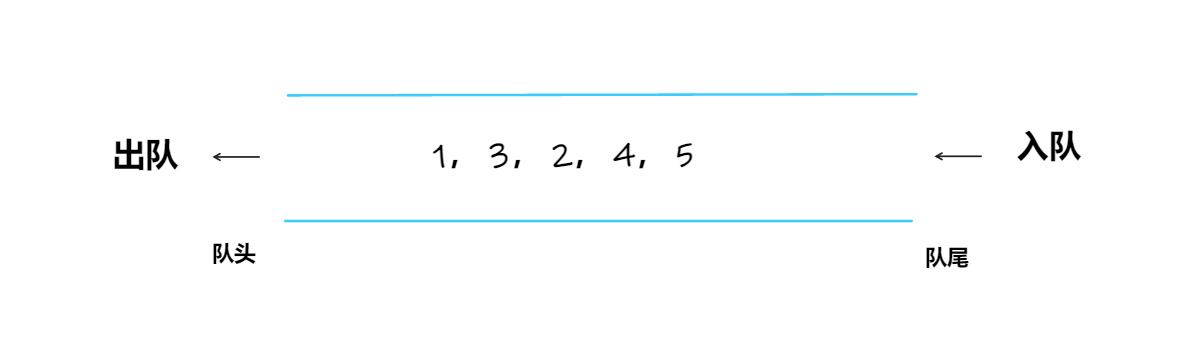
Stack, monotone stack, queue, monotone queue
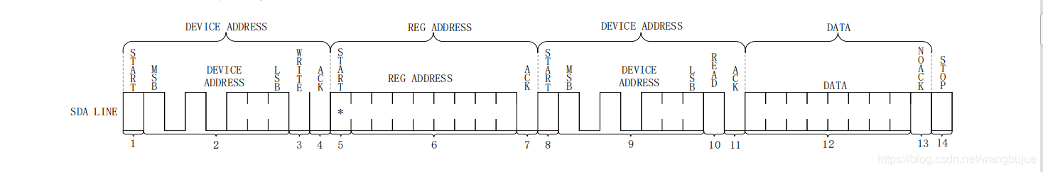
Driver development based on I2C protocol

Abandon the Internet after 00: don't want to enter a big factory after graduation, but go to the most fashionable Web3
2022 东北四省赛 VP记录/补题
随机推荐
在腾讯云容器服务Node上执行 kubectl
AMS series - application startup process
2022-07-02: what is the output of the following go language code? A: Compilation error; B:Panic; C:NaN。 package main import “fmt“ func mai
读书笔记:《心若菩提》 曹德旺
Solve undefined reference to`__ aeabi_ Uidivmod 'and undefined reference to`__ aeabi_ Uidiv 'error
The manuscript will be revised for release tonight. But, still stuck here, maybe what you need is a paragraph.
【obs】obs的ini格式的ConfigFile
Summary of interview questions (2) IO model, set, NiO principle, cache penetration, breakdown avalanche
1. Hal driven development
今晚要修稿子準備發佈。但是,仍卡在這裡,也許你需要的是一個段子。
After a month, I finally got Kingdee offer! Share tetrahedral Sutra + review materials
DS90UB949
【obs】封装obs实现采集的基础流程
After using the thread pool for so long, do you really know how to reasonably configure the number of threads?
2022 东北四省赛 VP记录/补题
Google Earth Engine(GEE)——GHSL 全球人口网格数据集250米分辨率
如何清理v$rman_backup_job_details视图 报错ORA-02030
(二)进制
Google Earth engine (GEE) - ghsl global population grid dataset 250 meter resolution
After setting up ADG, instance 2 cannot start ora-29760: instance_ number parameter not specified