November 9, 2020 [wgs/gwas] - whole genome analysis (association analysis) process (Part 2)

2021.07.30 Updated data analysis section ： Check me out.

One . Abstract

After a period of half a month patchwork R & D testing , The author has finally sorted out a VCF At the beginning GWAS Post analysis process . Of course, I would like to thank a lot of big guys for providing Code help , Reference links are also included in the article . Yes GWAS Friends who are not familiar enough , You can take a look at the one I sorted out before PPT Learning notes 《 Genetic evolution and GWAS Research 》.

Two . SNP Inspection and notes

Use software ：snpEff
Installation mode ：
miniconda3: conda install snpeff
SnpEff and SnpSift (pcingola.github.io)
Usage flow ：
Download the reference genome and annotation file （ Be careful vcf Chromosomes are numbers , Use RefSeq perhaps GenBank Numbering requires uniform chromosome sequence numbering ）

java -jar /home/yangxin/miniconda3/pkgs/snpeff-5.0-0/share/snpeff-5.0-0/snpEff.jar build -c /home/yangxin/miniconda3/pkgs/snpeff-5.0-0/share/snpeff-5.0-0/snpEff.config -gtf22 -v GCF_002163495.1_Omyk_1.0_genomic
# Parameter description 
#java -jar: Java Run the program in the environment 
#-c snpEff.config Profile path 
#-gff3  Set the input genome annotation information to gff3 Format , If it is gtf Please change the file to -gtf22
#-v  Set the log information output during program operation 

final -v Parameters Set the input genome version information , and snpEff.config The information added in the configuration file is consistent

java -jar /home/yangxin/miniconda3/pkgs/snpeff-5.0-0/share/snpeff-5.0-0/snpEff.jar build -c /home/yangxin/miniconda3/pkgs/snpeff-5.0-0/share/snpeff-5.0-0/snpEff.config -gff3 -v GCF_002163495.1_Omyk_1.0_genomic # Build a genome database 

Process chromosome numbers （ Optional ）
Because the genome I downloaded uses RefSeq Serial number , therefore , I need to change the chromosome number .

awk '{
    $1="";print $0}' OFS="\t" AxiomGT1.calls.vcf > col_2.vcf 
 If your chromosome is not consistent with the database , Then you can manually generate the chromosome sequence file col_chr2.vcf
paste -d '' col_chr2.vcf col_2.vcf >AxiomGT1.vcf # Merge sequence 
sed -n l AxiomGT1.vcf # Check vcf Whether the file format is consistent , Note that the separator is “\t”

Be careful ：cat、head、less I can't see the problem of the separator

java -jar ~/miniconda3/pkgs/snpeff-5.0-0/share/snpeff-5.0-0/snpEff.jar eff -c ~/miniconda3/pkgs/snpeff-5.0-0/share/snpeff-5.0-0/snpEff.config GCF_002163495.1_Omyk_1.0_genomic AxiomGT1.vcf > AxiomGT1.snp.eff.vcf -csvStats AxiomGT1_positive.csv -stats AxiomGT1_positive.html # Yes snp Annotate 
awk -F "|" '{print $1,$2,$4,$5,$8,$9}' OFS="\t" AxiomGT1.snp.eff.vcf > SNV.anno.xls # Generate comment file 
# Parameters -F "|" Used to process header information , If the header is normal, this parameter can be omitted 

Result display ： Notes file form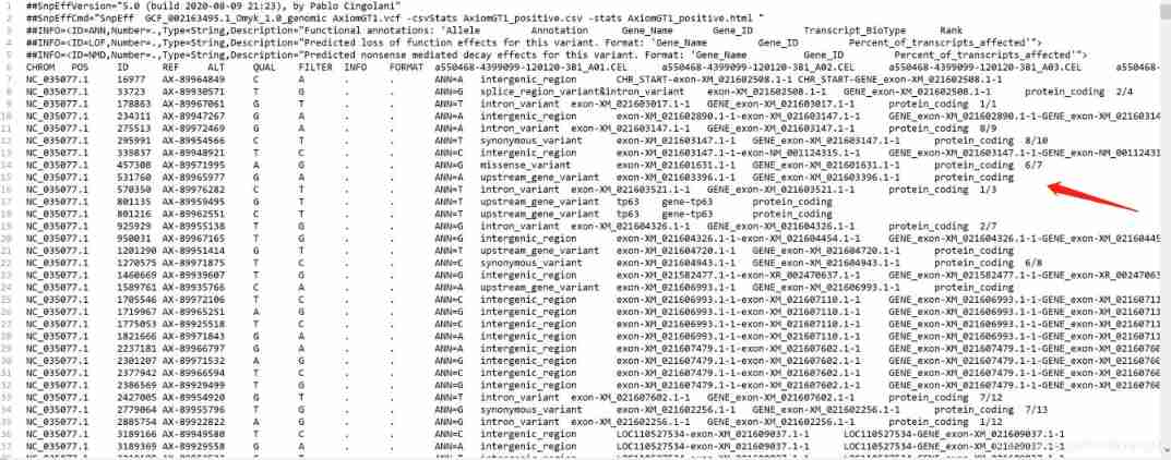
Process reference ：SnpEff Usage method

3、 ... and . Groups SNP Filter

Use software ：vcftools
Installation mode ：
miniconda3: conda install vcftools
Usage flow ：
Basic filter parameters Calling rate < 95%, Minor allele count < 3.

vcftools --vcf AxiomGT1.calls.vcf --max-missing 0.95 --mac 3 --recode --recode-INFO-all --out AxiomGT1.calls.filter.vcf
#--max-missing 0.95, The filter calling rate lower than 95％ The genotype of 
#--mac 3 Filter minor allele count less than 3 Of SNP

vcftools --vcf AxiomGT1.calls.filter.recode.vcf --missing-indv
# Test sample data loss rate , If the loss rate is too high, you need to adjust the parameters .
Result display
Before filtration ：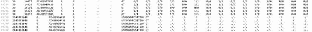
After filtration ：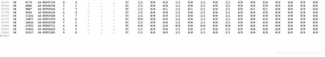

Four . Group stratified analysis

Group stratification refers to the existence of subgroups within a group , The interrelationship among individuals within a subgroup is greater than that among individuals within the entire population Average kinship . Between different subgroups , Some stable alleles have different frequencies , When two subgroups are mixed for association analysis Time analysis , Will lead to false positive results . therefore , Before performing correlation analysis , Be sure to carry out group stratification analysis first .

The group stratification analysis has ： Population evolutionary tree analysis and principal component analysis , The results of the two can be mutually verified .

4.1 Population evolutionary tree analysis

There are many software to draw the evolution tree , But after a few tests, I still feel tassel Visual interface drawing is the most convenient , Now let's introduce
Use software ：Tassel
Software installation ：miniconda3: conda install tassel5.0
Download from the official website ：Tassel (bitbucket.io)
Usage flow （ Visual drawing ）：
step1： open Tassel
step2： Import and open vcf file

step3： Create an evolution tree document

step4： Draw evolution tree

step5： Adjust the image

Function introduction ：
On the left side, you can add or delete parameters of the input file ;
The lower left corner X,Y± Used to adjust the length and width of the evolutionary tree ;
top left corner File You can output files in various formats ;
On the toolbar Type You can choose the type of evolutionary tree .（ The last circle is more beautiful ）
Result display

Be careful ： because VCF The file in Tassel There is a maximum character limit for association analysis , Just intercept the front 10 Characters , But drawing an evolutionary tree doesn't handle characters . So if you are worried that it is inconvenient to draw the evolution tree, you can handle it in advance .

Tassel The use of reference ：https://bitbucket.org/tasseladmin/tassel-5-source/wiki/UserManual
Manual in Chinese (2014)：https://wenku.baidu.com/view/4c0cabbe9b6648d7c0c746b2.html

4.2 Group principal component analysis

Use software ：Plink
Software installation ：miniconda3: conda install Plink
Usage flow ：

vcftools --vcf AxiomGT1.calls.vcf --plink --out GT1
# Generate plink Needed ped/map Format 
plink --file GT1 --make-bed --out GT1 --chr-set 30
# Convert to bed Format , Non human chromosomes , Use --chr-set Parameter setting chromosome number 
Plink --threads 8 --bfile snp --pca 10 --out pca
#--threads  Number of threads  --bfile  Input .bed file  --pca  The component of the principal component  --out Output file name 

###########R-PCA###########

mydat<-read.table("pca.eigenvec",as.is = T,header = T,stringsAsFactors = F)
png("PCA.png",width = 7000,height = 7000,pointsize = 160)

Result display

Tassel,GCTA perhaps EIGENSOFT It can also be analyzed , You can try more .

4.3 Population genetic structure analysis

In this part, I have a special article to introduce the use of error reporting , You can directly jump to the reference ：Admixture Population genetic structure analysis
Use software ：admixture
Software installation ：miniconda3: conda install admixture
Usage flow ：
The above is the same as the principal component analysis , Need to use plink take VCF File conversion to bed/bim/fam A few papers

vcftools --vcf AxiomGT1.calls.vcf --plink --out GT1
# Generate plink Needed ped/map Format 
plink --file GT1 --make-bed --out GT1 --chr-set 30
# Convert to bed Format , Non human chromosomes , Use --chr-set Parameter setting chromosome number 

Admixture Tool handling

for K in 2 3 4 5 6 7 8 9 10; \
do admixture --cv GT1_test.bed $K | tee log${K}.out; done
#2 3 4 5 6 7 8 9 10 The number of group structures divided  hapmap3.bed  Input file 
grep -h CV log*.out

# View best K value （ minimum value ）, Best output K Value file or show all K Worth the result
#R mapping

for (k in 2:10){
    
file_name = paste("GT1_test.",k,".Q",sep="")
result_name = paste(file_name,".PDF",sep="")
pdf(result_name,width=15,height=3)
tbl <- read.table(file_name,header = T)
barplot(t(as.matrix(tbl)), col=rainbow(k),xlab="Individual", ylab="Ancestry", border=NA)
dev.off()
}

Result display ：
With k=3,k=8 For example

5、 ... and . Linkage disequilibrium analysis

2018 year 10 month 15 Japan ,Bioinformatics The magazine published online PopLDdecay Software , Used to analyze the attenuation of linkage disequilibrium （Linkage disequilibrium (LD) decay）.PopLDdecay It can be read directly VCF file , Compared to calculating LD frequently-used PLINK Software , This feature simplifies the tedious process of format conversion .

Use software ：PopLDdecay

Source download ：PopLDdecay-3.41

Usage flow ：
If you want to plot by phenotype , We need to build a list, Calculate by phenotype ,list The format is a list of sample names of this phenotype

PopLDdecay -InVCF AxiomGT1.calls.vcf -OutStat RESISTANT -SubPop RESISTANT.list # Parting calculation 
gunzip RESiSTANT.stat.gz # Other phenotypic operations are the same 

Groups were established according to different phenotypes list, The single line format is stat route , Separator ,stat File prefix

perl ~/soft/PopLDdecay-3.41/bin/Plot_MultiPop.pl -inList file.list -output Fig

Result display

Reference link ：PopLDdecay: be based on VCF Fast file 、 A tool for efficiently calculating chain disequilibrium

6、 ... and . Select elimination analysis

Population evolutionary selection elimination analysis simply means that a region of the genome is selected to eliminate polymorphism . Selective elimination analysis is the imprint of positive selection on the genome of a species . Compared with the wild ancestors , The regional genetic diversity of cultivated or domesticated species is significantly reduced by selective elimination , This is a typical feature of domesticated areas .

Use software ：vcftools
Software installation ： A little

6.1 Fst analysis

The fixed coefficient of the group F It reflects the heterozygosity level of population alleles . Fixed coefficient F yes F statistic （Fst） A special case of .Fst The analysis indicates the degree of differentiation of the population , The bigger the value is. , The higher the degree of population differentiation , The more selective .

## For each SNP The variation sites were calculated 
vcftools --vcf AxiomGT1.calls.vcf --weir-fst-pop 1_population.txt --weir-fst-pop 2_population.txt  --out Fst_AximoGT1

## Calculate in steps 
vcftools --vcf test.vcf --weir-fst-pop 1_population.txt --weir-fst-pop 2_population.txt  --out p_1_2_bin --fst-window-size 500000 --fst-window-step 50000
#test.vcf yes SNP calling  Generated after filtering vcf  file ;
#p_1_2_3  Generate the result prefix
#1_population.txt It's a document , Include all individuals in group one , Usually one individual per line . The individual name should be the same as vcf The name of corresponds to .
#2_population.txt  It includes all the individuals in group 2 .
# The calculation window is 500kb, And the step size is 50kb （ It can be adjusted according to your needs ）. We can also calculate only for each point Fst, Remove the parameters （--fst-window-size 500000 --fst-window-step 50000） that will do .

#R-manhattan mapping

library(qq)
data<-read.table("Fst_AxiomGT1.weir.fst",header=T)
pdf(file="Fst_manhattan.pdf",width=20,height=8)
png(file="Fst_manhattan.png",width=2400,height=960)
#sc3 = subset(data,CHROM=="1")  Select any chromosome for analysis 
manhattan(data,chr="CHROM",bp="POS",p="WEIR_AND_COCKERHAM_FST",logp=F,main="Manhattan Plot",col = c("#8DA0CB","#E78AC3","#A6D854","#FFD92F","#E5C494","#66C2A5","#FC8D62"),annotatePval = 0.01)
dev.off()

Result display

6.2 θπ analysis

π To analyze base polymorphism , The lower the polymorphism , The more selective .

vcftools --vcf AxiomGT1.calls.vcf --keep RESISTANT.list --recode --out AxiomGT1.RESISTANT

vcftools --vcf AxiomGT1.calls.vcf --keep SUSCEPTIBLE.list --recode --out AxiomGT1.SUSCEPTIBLE_500K
# Classify the two phenotypes 

vcftools --vcf AxiomGT1.RESISTANT.recode.vcf --window-pi 500000 --window-pi-step 500000 --out AxiomGT1.RESISTANT_500K
# With 500K Calculate the step size separately pi value 

paste -d '\t' RESISTANT_typename.list AxiomGT1.RESISTANT_500K.windowed.pi > type_RESISTANT_500K.windowed.pi
# Create phenotype labels separately list, to windowed.pi The document is labeled with phenotype 

#R mapping

library(ggplot2)
data<-read.table("allsample_500K.windowed.pi",header=T)
for (i in 1:29){
    
#result_name = paste("chr",i,".pdf",sep="")
#pdf(result_name,width=15,height=3)
result_name = paste("chr",i,".png",sep="")
png(result_name,width=1500,height=300)
chrom = subset(data,CHROM==i)
xlab = paste("Chromosome",i,"(MB)",sep="")
p <- ggplot(chrom,aes(x=BIN_END/1000000,y=PI,group=Phenotype,color=Phenotype,shape=Phenotype)) + geom_line(size=0.5) + xlab(xlab)+ ylab("Pi") + theme_bw()
print(p)
dev.off()
}

Result display

7、 ... and . Genome wide association analysis

Genome wide association analysis （Genome-wide association study,GWAS） It is a common genetic variation in the whole genome （ Single nucleotide polymorphisms and copy numbers ） The method of gene association analysis , This method takes the natural population as the research object , With a gene that remains after long-term recombination （ site ） Linkage disequilibrium （linkage disequilibrium, LD） Based on , Combining phenotypic diversity of target traits with genes （ Or marker sites ） The polymorphisms of , It can be directly identified to be closely related to phenotypic variation A gene or marker site that is related and has a specific function . use GWAS Technology is studied on a genome-wide scale , It can locate multiple traits at one time , It is suitable for locating the correlation interval of traits 、 Functional gene research 、 Research on the development of trait breeding markers .
There are many software available for analysis , Such as GEMMA、Plink perhaps Tassel. The analysis method is also divided into general linear model and mixed linear model . Here we use GEMMA Analysis of cases .

7.1 Trait association analysis

Use software ：GEMMA
Source download ：Releases · genetics-statistics/GEMMA · GitHub
Usage flow ：

vcftools --vcf AxiomGT1.calls.vcf --plink --out GT1
# Generate plink Needed ped/map Format 
plink --file GT1 --make-bed --out GT1 --chr-set 30
# Convert to bed Format , Non human chromosomes , Use --chr-set Parameter setting chromosome number 
~/soft/gemma-0.98.1-linux-static -bfile GT1 -gk 2 -p p.txt
~/soft/gemma-0.98.1-linux-static -bfile GT1 -k output/result.sXX.txt -lmm 1 -p p.txt
#-bfile  Read plink Binary file （bed\bim\fam）
#-gk 2  Standardized method of calculation G matrix 
#-p  Read phenotype data （ Generate... Manually , It can't be omitted ）

The following uses the name qqman Of R Package drawing Manhattan map and qq chart , Download and install in advance

library(qqman) #  Load the package 
data <- read.table("result.assoc.txt",header = TRUE) # Reading data 
data1 <- data[,c(1,2,3,12)] # Intercept columns according to rules 
data2 <- na.omit(data1) #  Delete contains NA Entire line of 
par(cex=0.8) # Set point size 
#color_set <- rainbow(9)

The previous analysis steps are generic , Later, all chromosomes and single chromosomes were analyzed .

All chromosomes manhattan chart

#pdf(file="GWAS_manhattan.pdf", width=20, height=8)
png(file="GWAS_manhattan.png",width=2000, height=800)
manhattan(data2,chr="chr",snp="rs",bp="ps",p="p_wald",main="Manhattan Plot",col = c("#8DA0CB","#E78AC3","#A6D854","#FFD92F","#E5C494","#66C2A5","#FC8D62"),annotatePval = 0.01) #suggestiveline = FALSE  More significant 
dev.off() #  Save the picture 

Result display

A single chromosome manhattan chart

data <- read.table("result.assoc.txt",header = TRUE) # Reading data 
data1 <- data[,c(1,2,3,12)] # Intercept columns according to rules 
data2 <- na.omit(data1) #  Delete contains NA Entire line of 
par(cex=0.8) # Set point size 
for (i in 1:29){
    
result_name = paste("chr",i,".pdf",sep="")
pdf(result_name,width=15,height=6)
#result_name = paste("chr",i,".png",sep="")
#png(result_name,width=900,height=450)
chrom = subset(data2,chr==i)
main_title = paste("Chromosome",i,"(MB)",sep="")
manhattan(chrom,chr="chr",snp="rs",bp="ps",p="p_wald",main=main_title,col = c("#8DA0CB","#E78AC3","#A6D854","#FFD92F","#E5C494","#66C2A5","#FC8D62"),suggestiveline = FALSE, annotatePval = 0.01)
#suggestiveline = FALSE  Remove the difference significance line 
dev.off()
}

Result display

draw qq chart

pdf(file=“qqplot.pdf”, width=8, height=8)
png(file=“qqplot.png”)
qq(data2$p_wald) # draw qq chart
dev.off()
Result display

7.2 Multiple hypothesis test correction

Yes GEMMA Got result.assoc.txt Cut the document

awk '{print $2,$1,$3,$12}' result.assoc.txt >GWAS.adjust.xls

stay excel According to the P Value to find the correction value , The specific operations are as follows: p Sort values in ascending order , The correction value formula is ,FDR=p*m/k ,m by snp total ,k For the current snp ranking .
Result display

7.3 Notes on gene function of target trait related regions

adopt gwas4d Make online comments （ Then I will write a separate article to explain ）
Result display

Reference link ： The root is red and the seedling is positive GWAS Analysis software ：GEMMA_ Deng Fei ---- Analysis of breeding data -CSDN Blog

8、 ... and . Conclusion

Compared with the process of collecting references for half a month , This article has made some supplements and improvements . However , There is still a lot of room for optimization in all aspects , therefore , It's just a 1.0 edition , If there is a problem with the process , Or offer better advice , When the QR code expires, you can add VX：bbplayer2021 , remarks Apply to join the student information exchange group .

Nine . Reference link

SnpEff Usage method ：https://www.jianshu.com/p/a6e46d0c07ee
Tassel The use of reference ：https://bitbucket.org/tasseladmin/tassel-5-source/wiki/UserManual
Tassel Manual in Chinese (2014)：https://wenku.baidu.com/view/4c0cabbe9b6648d7c0c746b2.html
PopLDdecay: be based on VCF Fast file 、 A tool for efficiently calculating chain disequilibrium :http://wap.sciencenet.cn/blog-656335-1168505.html
The root is red and the seedling is positive GWAS Analysis software ：GEMMA_ Deng Fei ---- Analysis of breeding data -CSDN Blog https://blog.csdn.net/yijiaobani/article/details/106215223