当前位置:网站首页>[six articles talk about scalablegnn] around www 2022 best paper PASCA
[six articles talk about scalablegnn] around www 2022 best paper PASCA
2022-07-25 13:09:00 【chad_ lee】
Scalable GNN
《Simplifying Graph Convolutional Networks》 ICML 2019
《SIGN: Scalable Inception Graph Neural Networks》 ICML 2020 workshop
《Simple Spectral Graph Convolution》ICLR 2020
《Scalable and Adaptive Graph Neural Networks with Self-Label-Enhanced training》 arxiv’21 OGB Once the first place
《Graph Attention Multi-Layer Perceptron》 arxiv‘21 The same author
《PaSca: a Graph Neural Architecture Search System under the Scalable Paradigm》 WWW 2022 best paper
existing GNN The defects of
High Memory Cost
GNN Feature propagation operations in ( Neighbor aggregation mechanism 、 Message passing mechanism ) Involving the multiplication of a large sparse matrix and characteristic matrix , It takes more time ; If used during training GPU Speed up , Then we must put the matrix in GPU On the memory of , But this demand cannot be satisfied for the big picture . such as OGB The largest in the node classification dataset ogb The sparse adjacency matrix size of the dataset exceeds 50GB, At present, only 80GB Video memory version Tesla A100 To save , But you can use 250GB Memory operation , The latter is easier to get . So only distributed training GNN, But this will bring a lot
High Communication Cost
GNN Every feature propagation needs to aggregate neighbor features , about K Layer of GNN Come on , Each node needs to aggregate K Characteristics of neighbor nodes within hops , The number of nodes involved increases exponentially as the number of layers increases , This will bring a lot of communication overhead in distributed scenarios . For dense connected graphs , Each node almost needs to aggregate the node information of the whole graph every time it is trained . Some sampling algorithms (GraphSAGE) Can alleviate this problem , But because of the recursive neighbor aggregation mechanism in the training process , These algorithms still cause high communication costs .
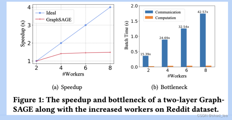
It can be seen that the performance bottleneck is the communication overhead , Add GPU Can't effectively speed up training .
Inconsistent Receptive Field expansion speed

The receptive field expansion speed of different nodes is different , Therefore, the optimal receptive field of different nodes is also different . chart a Is random 20 Test results of nodes , use SGC( Only the first K Layer of feature) Experiments done , Record continuous operation 100 Proportion of predicted correct times in total times . It can be seen that the prediction accuracy of different nodes varies with the increase of feature propagation steps , Such as node 10, The number of propagation steps is 1 The maximum prediction accuracy is reached , Subsequently, the prediction accuracy decreased continuously ; And there are some nodes , Such as node 4, The prediction accuracy increases with the increase of feature propagation steps . Even if the trend is the same , The optimal convolution layers of different nodes are also different . Therefore, when the node characteristics of different propagation steps are weighted and summed , Different weights should be given .
Different tasks need to be designed separately GNN structure
The existing GNN Work is to design a model structure , In different mission scenarios ( Data sets ) Domain experts may be required to design specific model structures 、 The training process , Modeling costs are high .
Scalable GNN summary
The article first summarizes Scalable GNN Architectural paradigm .Sampling-based The method is not Scalable GNN, Because these models also need to aggregate neighbor nodes in the training process , Communication overhead cannot be avoided in distributed scenarios .
model decoupling
Some research points out that 【SGC】,GNN The performance of is mainly due to the feature propagation operation in each layer , Instead of nonlinear transformation operation . This gave birth to a series of decoupling GNN, They are designing GNN The feature propagation operation and nonlinear transformation operation are decoupled , All feature propagation operations are completed in advance during preprocessing , In model training, there is no need to spend time and effort to propagate features . therefore , In terms of scalability , As long as the sparse matrix and dense matrix multiplication in the feature propagation operation can be completed during preprocessing , The subsequent model training can be easily carried out on a single machine and a single card . Because the feature propagation operation is completed in the preprocessing process , Therefore, there is no need to use GPU Accelerate , You can use only CPU Perform matrix multiplication .
But these are decoupled GNN The specificity of different nodes was not distinguished during training .SIGN、S2GC、SAGN、GAMLP We consider specificity .
SGC—— Consider only the K Characteristics of the layer
《Simplifying Graph Convolutional Networks》 ICML‘19

In the pretreatment stage ,SGC use K-step Features obtained after feature propagation ( Only the first K Output of layer convolution ), As the initial feature of the node : X ‾ ← S K X \overline{\mathbf{X}} \leftarrow \mathbf{S}^{K} \mathbf{X} X←SKX, S \mathbf{S} S It's an adjacency matrix . Then only one is trained in the model training stage 1 Layer of MLP As a classifier .
SIGN—— Consider different receptive fields
《SIGN: Scalable Inception Graph Neural Networks》 ICML‘20 workshop
SGC It only took K-step The obtained feature is used as the initial feature of the node , Obviously, it is not optimal for all nodes ,SIGN take 0~K-step All the features are stitched together , It retains the characteristics of all receptive fields :
Z = σ ( [ X Θ 0 , A 1 X Θ 1 , … , A r X Θ r ] ) Y = ξ ( Z Ω ) \begin{aligned} \mathbf{Z} &=\sigma\left(\left[\mathbf{X} \boldsymbol{\Theta}_{0}, \mathbf{A}_{1} \mathbf{X} \boldsymbol{\Theta}_{1}, \ldots, \mathbf{A}_{r} \mathbf{X} \boldsymbol{\Theta}_{r}\right]\right) \\ \mathbf{Y} &=\xi(\mathbf{Z} \boldsymbol{\Omega}) \end{aligned} ZY=σ([XΘ0,A1XΘ1,…,ArXΘr])=ξ(ZΩ)
Θ \boldsymbol{\Theta} Θ and Ω \boldsymbol{\Omega} Ω All training parameters . The disadvantage is that the space cost of splicing is directly proportional to the number of convolution layers .
S2GC——PPR+ Average
《Simple Spectral Graph Convolution》ICLR‘20

Y ^ = softmax ( 1 K ∑ k = 1 K ( ( 1 − α ) T ~ k X + α X ) W ) \hat{Y}=\operatorname{softmax}\left(\frac{1}{K} \sum_{k=1}^{K}\left((1-\alpha) \tilde{\mathbf{T}}^{k} \mathbf{X}+\alpha \mathbf{X}\right) \mathbf{W}\right) Y^=softmax(K1k=1∑K((1−α)T~kX+αX)W)
T T T Or adjacency matrix ,S2GC In fact, it is approximate in probability ( 1 − α 1-\alpha 1−α) Rebooted PPR Get the characteristics of each layer , And then add them evenly , As the initial feature of the node .
SAGN—— Different receptive fields attention Sum up
《Scalable and Adaptive Graph Neural Networks with Self-Label-Enhanced training》 arxiv’21

hold SIGN The splicing operation in is replaced by attention Weighted sum of , Weighted sum of different receptive field characteristics , Later articles are follow This paradigm .
GAMLP—— Design attention
《Graph Attention Multi-Layer Perceptron》 arxiv‘21

1、Smoothing Attention
It can be understood as the node feature after infinite times of feature propagation X i ( ∞ ) X_{i}^{(\infty)} Xi(∞) As reference vector , And then calculate attention:
X ~ i ( l ) = X i ( l ) ∥ X i ( ∞ ) , w ~ i ( l ) = δ ( X ~ i ( l ) ⋅ s ) , w i ( l ) = e w ~ i ( l ) / ∑ k = 0 K e w ~ i ( k ) \widetilde{\mathbf{X}}_{i}^{(l)}=\mathbf{X}_{i}^{(l)} \| \mathbf{X}_{i}^{(\infty)}, \quad \widetilde{w}_{i}(l)=\delta\left(\tilde{\mathbf{X}}_{i}^{(l)} \cdot s\right), \quad w_{i}(l)=e^{\widetilde{w}_{i}(l)} / \sum_{k=0}^{K} e^{\widetilde{w}_{i}(k)} Xi(l)=Xi(l)∥Xi(∞),wi(l)=δ(X~i(l)⋅s),wi(l)=ewi(l)/k=0∑Kewi(k)
among s ∈ R 1 × d s \in \mathbb{R}^{1 \times d} s∈R1×d It's a trainable parameter . The larger w i ( l ) w_{i}(l) wi(l) It means that nodes v i v_{i} vi Of l-step The propagation characteristics are far away from the infinite propagation state , The risk of becoming noise is small . With larger w i ( l ) w_{i}(l) wi(l) The transmission characteristics of should contribute more to the combination of characteristics .
2、Recursive Attention
Recursively calculate the information gain in the process of feature propagation :
X ~ i ( l ) = X i ( l ) ∥ ∑ k = 0 l − 1 w i ( k ) X i ( k ) , w ~ i ( l ) = δ ( X ~ i ( l ) ⋅ s ) , w i ( l ) = e w ~ i ( l ) / ∑ k = 0 K e w ~ i ( k ) \tilde{\mathbf{X}}_{i}^{(l)}=\mathbf{X}_{i}^{(l)} \| \sum_{k=0}^{l-1} w_{i}(k) \mathbf{X}_{i}^{(k)}, \tilde{w}_{i}(l)=\delta\left(\tilde{\mathbf{X}}_{i}^{(l)} \cdot s\right), w_{i}(l)=e^{\tilde{w}_{i}(l)} / \sum_{k=0}^{K} e^{\tilde{w}_{i}(k)} X~i(l)=Xi(l)∥∑k=0l−1wi(k)Xi(k),w~i(l)=δ(X~i(l)⋅s),wi(l)=ew~i(l)/∑k=0Kew~i(k)
The larger w i ( l ) w_{i}(l) wi(l) Signifying characteristics X i ( l ) \mathbf{X}_{i}^{(l)} Xi(l) Yes v i v_{i} vi The current state of is more important ( Compared with the previous layer, the combination features account for a higher proportion ).
3、JK Attention

Will all step Feature input to MLP,MLP The output result is used as the reference vector , Calculation attention:
X ~ i ( l ) = X i ( l ) ∥ E i , w ~ i ( l ) = δ ( X ~ i ( l ) ⋅ s ) , w i ( l ) = e w ~ i ( l ) / ∑ k = 0 K e w ~ i ( k ) E i = M L P ( X i ( 1 ) ∥ X i ( 2 ) ∥ … ∥ X i ( K ) ) \tilde{X}_{i}^{(l)}=X_{i}^{(l)} \| E_{i}, \quad \widetilde{w}_{i}(l)=\delta\left(\tilde{X}_{i}^{(l)} \cdot \mathrm{s}\right), \quad w_{\mathrm{i}}(l)=e^{\widetilde{w}_{i}(l)} / \sum_{k=0}^{K} e^{\widetilde{w}_{i}(k)} \\ \mathbf{E}_{i}=\mathbf{M L P}\left(\mathbf{X}_{i}^{(1)}\left\|\mathbf{X}_{i}^{(2)}\right\| \ldots \| \mathbf{X}_{i}^{(K)}\right) X~i(l)=Xi(l)∥Ei,wi(l)=δ(X~i(l)⋅s),wi(l)=ewi(l)/k=0∑Kewi(k)Ei=MLP(Xi(1)∥∥Xi(2)∥∥…∥Xi(K))
Scalable GNN Model design space
《PaSca: a Graph Neural Architecture Search System under the Scalable Paradigm》 WWW 2022 best paper
As mentioned above Scalable GNN Are a specific model architecture , According to the above work , It can be concluded that Scalable GNN Model design space , Then you can define the search target ( Accuracy and speed ), Search for the one that is suitable for the current task scenario Scalable GNN.
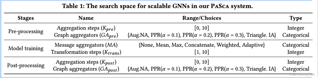
Scalable GNN The model design of can be divided into three stages :
1、 Pretreatment stage
Aggregation step( K p r e K_{pre} Kpre) It refers to the feature obtained by convolution of several layers at most .
Graph aggregator( G A p r e GA_{pre} GApre) It refers to the adjacency matrix used by the neighbor aggregation mechanism , For example, after standardization A、PPR etc. .
It's described above SGC、SIGN、SAGN、GAMLP It's used A;S2GC It's using PPR.
2、 Model training stage
Message aggregators( M A MA MA) It refers to how to use the obtained k-steps Characteristics of .None Only the last layer (SGC);Mean Namely S2GC;Concatenate Namely SIGN;Weighted Namely SAGN;Adaptive Namely GAMLP. It's not good to use only one layer , Because different nodes have different optimal receptive fields .
Transformation step( K t r a n s K_{trans} Ktrans) Refer to MLP The number of layers .
3、 Post processing stage
there K p o s K_{pos} Kpos and G A p o s t GA_{post} GApost And pretreatment stage K p r e K_{pre} Kpre and G A p r e GA_{pre} GApre identical , The purpose is to Label Propagation, The model predicts Classification probability distribution Spread it several times , Be similar to APPNP, But it is directly transmitted to the model output after training .

The whole model design space contains 18 Ten thousand model architectures , The above summary Scalable GNN Are concrete examples of this design space :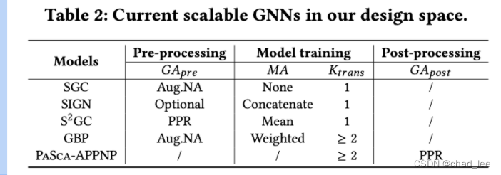
Model structure automatic search system ( Auto search super parameter )

This part of the article is very short . It is divided into two engines : One is the search engine , One is the evaluation engine .
Search engine is based on Bayesian optimization to realize the recommendation of model structure . First, define the optimization objective : Accuracy and training speed . Then model the relationship between the observed model structure and the optimization goal ( Try to establish a mapping ), Return a model structure that can balance multiple optimization objectives , Let the evaluation engine verify .
The evaluation engine is to train the model , Then return the results to the search engine , In this way, there is another observation result of search engine .
experimental result
Communication overhead
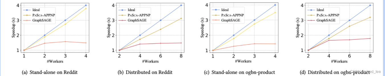
Model accuracy and efficiency :

PaSca The found model can better balance the training efficiency and model accuracy . It can be seen from the right figure that there is no decoupling GCN Compared with decoupling GCN, Performance has no significant advantage , But the efficiency is more than 100 times worse .

ScalableGNN No, over-smoothing, Because the output of deep convolution is used as an initial feature ,Attention You can pay attention or not .
边栏推荐
- 【运维、实施精品】月薪10k+的技术岗位面试技巧
- [figure attack and Defense] backdoor attacks to graph neural networks (sacmat '21)
- Lu MENGZHENG's "Fu of broken kiln"
- 深度学习的训练、预测过程详解【以LeNet模型和CIFAR10数据集为例】
- Docekr学习 - MySQL8主从复制搭建部署
- The world is exploding, and the Google server has collapsed
- Handwriting a blog platform ~ first day
- 零基础学习CANoe Panel(13)—— 滑条(TrackBar )
- 迁移PaloAlto HA高可用防火墙到Panorama
- 【AI4Code】《CodeBERT: A Pre-Trained Model for Programming and Natural Languages》 EMNLP 2020
猜你喜欢
![[ai4code final chapter] alphacode: competition level code generation with alphacode (deepmind)](/img/05/86eed30a7c063beace400a005e4a4c.png)
[ai4code final chapter] alphacode: competition level code generation with alphacode (deepmind)

【CSDN 年终总结】结束与开始,一直在路上—— “1+1=王”的2021总结

微软提出CodeT:代码生成新SOTA,20个点的性能提升

错误: 找不到或无法加载主类 xxxx

Convolutional neural network model -- alexnet network structure and code implementation

Redis可视化工具RDM安装包分享
好友让我看这段代码

卷积核越大性能越强?一文解读RepLKNet模型
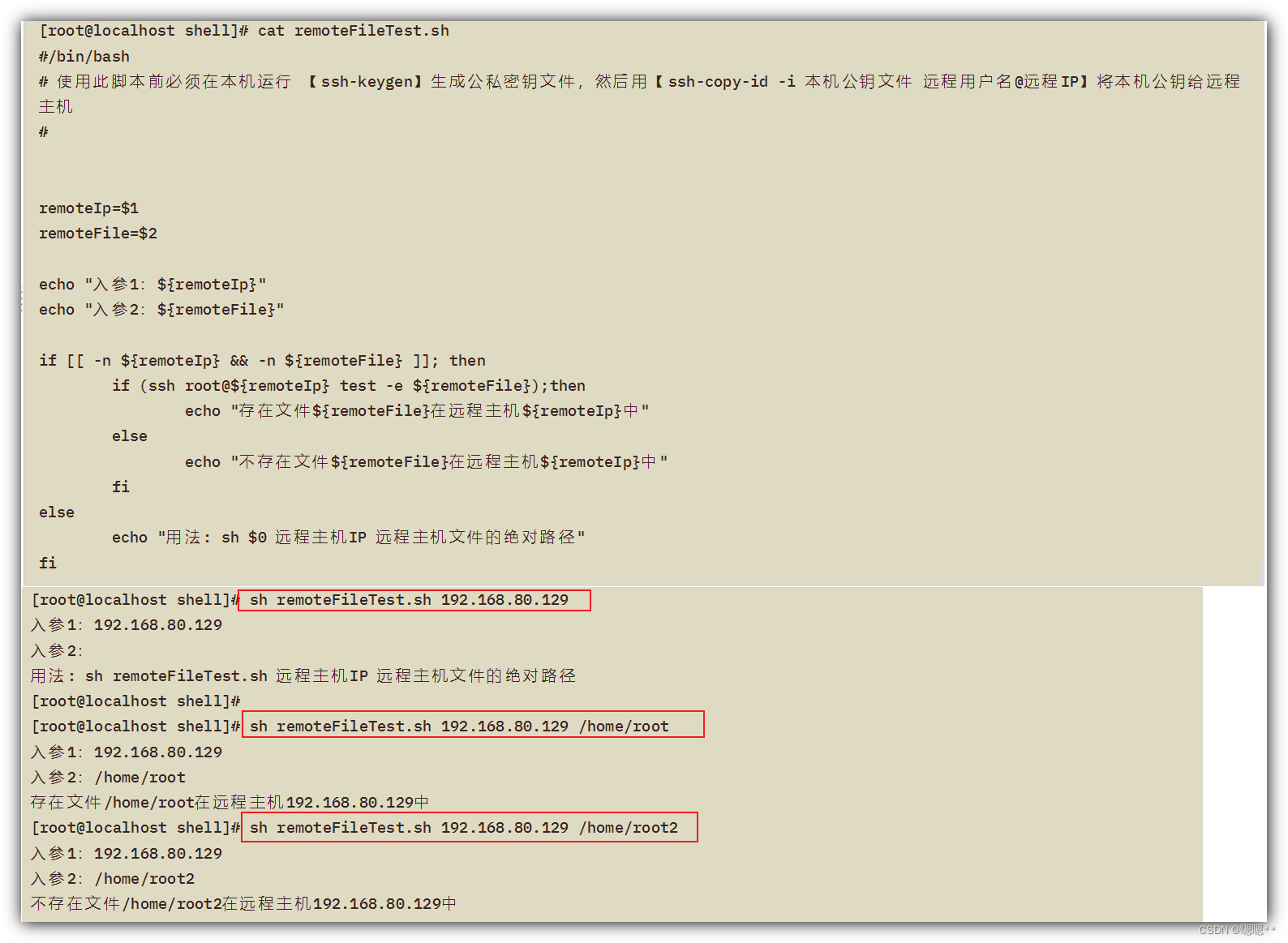
Shell common script: judge whether the file of the remote host exists

EMQX Cloud 更新:日志分析增加更多参数,监控运维更省心
随机推荐
[ai4code final chapter] alphacode: competition level code generation with alphacode (deepmind)
【视频】马尔可夫链原理可视化解释与R语言区制转换MRS实例|数据分享
Zero basic learning canoe panel (13) -- trackbar
Use of Spirng @conditional conditional conditional annotation
Substance designer 2021 software installation package download and installation tutorial
Chapter5 : Deep Learning and Computational Chemistry
The programmer's father made his own AI breast feeding detector to predict that the baby is hungry and not let the crying affect his wife's sleep
[review SSM framework series] 15 - Summary of SSM series blog posts [SSM kill]
简单了解流
Shell common script: check whether a domain name and IP address are connected
Shell常用脚本:获取网卡IP地址
手写一个博客平台~第一天
【OpenCV 例程 300篇】239. Harris 角点检测之精确定位(cornerSubPix)
Make a general cascade dictionary selection control based on jeecg -dictcascadeuniversal
如何用因果推断和实验驱动用户增长? | 7月28日TF67
I want to ask whether DMS has the function of regularly backing up a database?
零基础学习CANoe Panel(16)—— Clock Control/Panel Control/Start Stop Control/Tab Control
2022 年中回顾 | 大模型技术最新进展 澜舟科技
【AI4Code】《CodeBERT: A Pre-Trained Model for Programming and Natural Languages》 EMNLP 2020
【CSDN 年终总结】结束与开始,一直在路上—— “1+1=王”的2021总结