1、生成对抗网络入门

GAN简介（Generative Adversarial Nets）

小偷（Generator Network）通过随机变量（Random Vector）生成假钱（Fake Image）存进银行（Discriminator Network），银行通过真钱（Real Image）、假钱（Fake Image）学习判断小偷的假钱，循环上述步骤。

小偷希望银行判断假钱为真钱，所以将假钱（标签值为真）交给银行判断，得到银行反馈的loss，以此进行更新迭代，优化造假技术

银行希望准确判断真假币，所以同时对小偷的假钱（标签值为假）、和训练的真钱（标签值为真）进行训练，以此进行更新迭代

损失函数

import torch
from torch import autograd
import torch.nn as nn
import math

input = autograd.Variable(torch.tensor([
    [1.9072, 1.1079, 1.4906],
    [-0.6548, -0.0512, 0.7608],
    [-0.0614, 0.6583, 0.1095]
]))
print(input)
print('-' * 100)

m = nn.Sigmoid()
print(m(input))
print('-' * 100)

target = torch.FloatTensor([
    [0, 1, 1],
    [1, 1, 1],
    [0, 0, 0]
])
print(target)
print('-' * 100)

r11 = 0 * math.log(0.8707) + (1 - 0) * math.log((1 - 0.8707))
r12 = 1 * math.log(0.7517) + (1 - 1) * math.log((1 - 0.7517))
r13 = 1 * math.log(0.8162) + (1 - 1) * math.log((1 - 0.8162))

r21 = 1 * math.log(0.3419) + (1 - 1) * math.log((1 - 0.3419))
r22 = 1 * math.log(0.4872) + (1 - 1) * math.log((1 - 0.4872))
r23 = 1 * math.log(0.6815) + (1 - 1) * math.log((1 - 0.6815))

r31 = 0 * math.log(0.4847) + (1 - 0) * math.log((1 - 0.4847))
r32 = 0 * math.log(0.6589) + (1 - 0) * math.log((1 - 0.6589))
r33 = 0 * math.log(0.5273) + (1 - 0) * math.log((1 - 0.5273))

r1 = -(r11 + r12 + r13) / 3
r2 = -(r21 + r22 + r23) / 3
r3 = -(r31 + r32 + r33) / 3

bceloss = (r1 + r2 + r3) / 3
print(bceloss)
print('-' * 100)


# torch 需要Sigmoid
loss = nn.BCELoss()
print(loss(m(input), target))
print('-' * 100)

# torch 不需要Sigmoid
loss = nn.BCEWithLogitsLoss()
print(loss(input, target))
print('-' * 100)

CycleGan

简介

• 实现效果

• 无须配对数据

• 如何学习
  
  生成器Gab通过真斑马生成假马，假马通过Gba生成假斑马，假斑马与真斑马产生L2损失，迭代优化

• 整体网络架构
  

• PatchGAN
  

入门测试

• 源码地址

https://github.com/junyanz/pytorch-CycleGAN-and-pix2pix

• 数据下载
  以文本形式打开文件
  
  复制下载链接
  
  
• 训练好的参数权重
  

https://github.com/junyanz/pytorch-CycleGAN-and-pix2pix/blob/master/scripts/download_cyclegan_model.sh#L3

http://efrosgans.eecs.berkeley.edu/cyclegan/pretrained_models/

将下载好的horse2zebra.pth文件放到pytorch-CycleGAN-and-pix2pix-master\checkpoints\horse2zebra_pretrained下，并修改名称为latest_net_G.pth

• 启动测试

测试参数

--dataroot datasets/horse2zebra/testA
--name horse2zebra.pth_pretrained
--model test --no_dropout
# 使用cpu
--gpu_ids -1

在pytorch-CycleGAN-and-pix2pix-master\results\horse2zebra_pretrained\test_latest下保存结果

打开index.html

visdom

CycleGan训练时使用visdom作为可视化工具，训练前先启动visdom

pip install visdom
python -m visdom.server

stargan

• 何为star

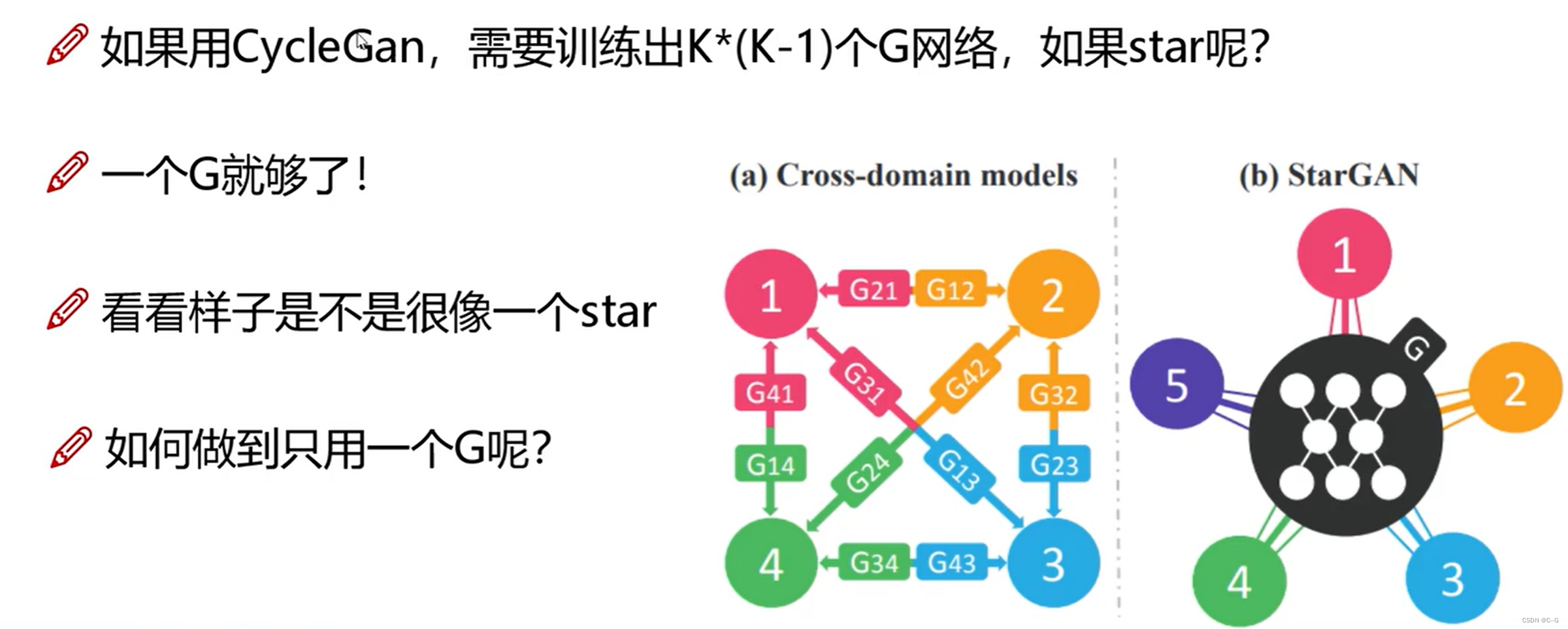
• 基本思路
  
• 整体流程
  
  
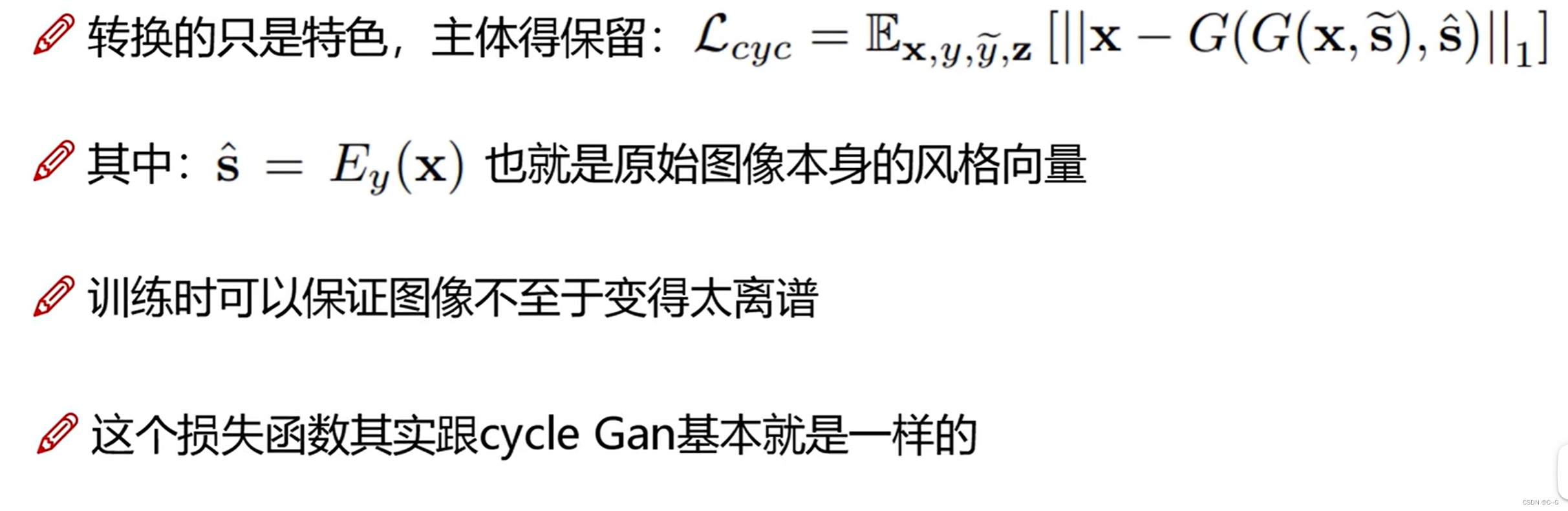
  输入图片与编码特征，通过生成器得到假照片，再将假照片通过生成器得到真实照片，并与原图进行对比，缩小真实照片与原图的差距

stargan使用编码代替风格，特征性不强，没有参与计算

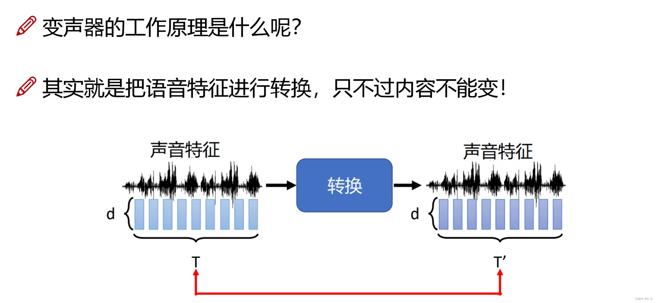
• 扩展：变声器
  

stargan-v2

• 整体网络架构
  
• 编码器训练（Style reconstruction）

• 多样化训练（Style diversification）
  
• cycle loss

代码分析

• 源码下载
  https://github.com/clovaai/stargan-v2
• 导入必须的包

conda create -n stargan-v2 python=3.6.7
conda activate stargan-v2
conda install -y pytorch=1.4.0 torchvision=0.5.0 cudatoolkit=10.0 -c pytorch
conda install x264=='1!152.20180717' ffmpeg=4.0.2 -c conda-forge
pip install opencv-python==4.1.2.30 ffmpeg-python==0.2.0 scikit-image==0.16.2
pip install pillow==7.0.0 scipy==1.2.1 tqdm==4.43.0 munch==2.5.0

• 生成器

class Generator(nn.Module):
    def __init__(self, img_size=256, style_dim=64, max_conv_dim=512, w_hpf=1):
        super().__init__()
        dim_in = 2**14 // img_size
        self.img_size = img_size
        self.from_rgb = nn.Conv2d(3, dim_in, 3, 1, 1)
        self.encode = nn.ModuleList()
        self.decode = nn.ModuleList()
        self.to_rgb = nn.Sequential(
            nn.InstanceNorm2d(dim_in, affine=True),
            nn.LeakyReLU(0.2),
            nn.Conv2d(dim_in, 3, 1, 1, 0))

        # down/up-sampling blocks
        repeat_num = int(np.log2(img_size)) - 4
        if w_hpf > 0:
            repeat_num += 1
        for _ in range(repeat_num):
            dim_out = min(dim_in*2, max_conv_dim)
            self.encode.append(
                ResBlk(dim_in, dim_out, normalize=True, downsample=True))
            self.decode.insert(
                0, AdainResBlk(dim_out, dim_in, style_dim,
                               w_hpf=w_hpf, upsample=True))  # stack-like
            dim_in = dim_out

        # bottleneck blocks
        for _ in range(2):
            self.encode.append(
                ResBlk(dim_out, dim_out, normalize=True))
            self.decode.insert(
                0, AdainResBlk(dim_out, dim_out, style_dim, w_hpf=w_hpf))

        if w_hpf > 0:
            device = torch.device(
                'cuda' if torch.cuda.is_available() else 'cpu')
            self.hpf = HighPass(w_hpf, device)

    def forward(self, x, s, masks=None):
        x = self.from_rgb(x)
        cache = {
    }
        for block in self.encode:
            if (masks is not None) and (x.size(2) in [32, 64, 128]):
                cache[x.size(2)] = x
            x = block(x)
        for block in self.decode:
            x = block(x, s)
            if (masks is not None) and (x.size(2) in [32, 64, 128]):
                mask = masks[0] if x.size(2) in [32] else masks[1]
                mask = F.interpolate(mask, size=x.size(2), mode='bilinear')
                x = x + self.hpf(mask * cache[x.size(2)])
        return self.to_rgb(x)

归一化层，目前主要有这几个方法，Batch Normalization（2015年）、Layer Normalization（2016年）、Instance Normalization（2017年）、Group Normalization（2018年）、Switchable Normalization（2018年）；

将输入的图像shape记为[N, C, H, W]，这几个方法主要的区别就是在，

• batchNorm是在batch上，对NHW做归一化，对小batchsize效果不好；
• layerNorm在通道方向上，对CHW归一化，主要对RNN作用明显；
• instanceNorm在图像像素上，对HW做归一化，用在风格化迁移；
• GroupNorm将channel分组，然后再做归一化；
• SwitchableNorm是将BN、LN、IN结合，赋予权重，让网络自己去学习归一化层应该使用什么方法。

• 风格特征编码

class MappingNetwork(nn.Module):
    def __init__(self, latent_dim=16, style_dim=64, num_domains=2):
        super().__init__()
        layers = []
        layers += [nn.Linear(latent_dim, 512)]
        layers += [nn.ReLU()]
        for _ in range(3):
            layers += [nn.Linear(512, 512)]
            layers += [nn.ReLU()]
        self.shared = nn.Sequential(*layers)

        self.unshared = nn.ModuleList()
        for _ in range(num_domains):
            self.unshared += [nn.Sequential(nn.Linear(512, 512),
                                            nn.ReLU(),
                                            nn.Linear(512, 512),
                                            nn.ReLU(),
                                            nn.Linear(512, 512),
                                            nn.ReLU(),
                                            nn.Linear(512, style_dim))]

    def forward(self, z, y):
        h = self.shared(z)
        out = []
        for layer in self.unshared:
            out += [layer(h)]
        out = torch.stack(out, dim=1)  # (batch, num_domains, style_dim)
        idx = torch.LongTensor(range(y.size(0))).to(y.device)
        s = out[idx, y]  # (batch, style_dim)
        return s

• 判别器

class Discriminator(nn.Module):
    def __init__(self, img_size=256, num_domains=2, max_conv_dim=512):
        super().__init__()
        dim_in = 2**14 // img_size
        blocks = []
        blocks += [nn.Conv2d(3, dim_in, 3, 1, 1)]

        repeat_num = int(np.log2(img_size)) - 2
        for _ in range(repeat_num):
            dim_out = min(dim_in*2, max_conv_dim)
            blocks += [ResBlk(dim_in, dim_out, downsample=True)]
            dim_in = dim_out

        blocks += [nn.LeakyReLU(0.2)]
        blocks += [nn.Conv2d(dim_out, dim_out, 4, 1, 0)]
        blocks += [nn.LeakyReLU(0.2)]
        blocks += [nn.Conv2d(dim_out, num_domains, 1, 1, 0)]
        self.main = nn.Sequential(*blocks)

    def forward(self, x, y):
        out = self.main(x)
        out = out.view(out.size(0), -1)  # (batch, num_domains)
        idx = torch.LongTensor(range(y.size(0))).to(y.device)
        out = out[idx, y]  # (batch)
        return out

stargan-vc2

http://www.kecl.ntt.co.jp/people/kaneko.takuhiro/projects/stargan-vc2/index.html

• 变声器

• 输入数据
  

• 预处理
  

• 特征汇总
  

• MFCC
  

• 生成器
  

• 语言数据包含的成分
  

• Instance Normalization 和 Adaptive Instance Normalization
  

• Instance Normalization
  
  内容编码器只需要内容，不需要语言特征，所以使用Instance Normalization对每个特征图进行归一化，将声音特征平均化，去掉语言特性

• AdaIn
  
  In归一化去掉了语言特征，AdaIn则是通过额外的FC层赋予语言特征

• PixelShuffle
  上采样与下采样：都是老路子，stride=2来下采样，反卷积来上采样
  **PixelShuffle层又名亚像素卷积层，是论文Real-Time Single Image and Video Super-Resolution Using an Efficient Sub-Pixel Convolutional Neural Network中介绍的一种应用于超分辨率重建应用的具有上采样功能的卷积层。这篇ESPCN论文介绍了这种层的功能，sub-pixel convolution layer以stride = 1 r stride=\frac{1}{r}stride= r1 (r rr为SR的放大倍数upscaling factor)去提取feature map，虽然称之为卷积，但是其并没用用到任何需要学习的参数，它的原理也很简单，就是将输入feature map进行像素重组，也就是说亚像素卷积层虽用卷积之名，但却没有做任何乘加计算，只是用了另一种方式去提取特征罢了：
  **

如上图所示的最后一层就是亚像素卷积层，它就是将输入格式为( b a t c h , r 2 C , H , W ) (batch,r^2C, H, W)(batch,r 2C,H,W)的feature map中同一通道的像素提取出来作为输出feature map的一小块，遍历整个输入feature map就可以得到最后的输出图像。整体来看，就好像是用1r\frac{1}{r}r1的步长去做卷积一样，这样就造成了不是对整像素点做卷积，而是对亚像素做卷积，故称之为亚像素卷积层，最后的输出格式就是( b a t c h , 1 , r H , r W ) (batch,1, rH,rW)(batch,1,rH,rW)。

因此，简单一句话，PixelShuffle层做的事情就是将输入feature map像素重组输出高分辨率的feature map，是一种上采样方法，具体表达为

其中r为上采样倍率(上图中r = 3)

• 判别器
  

图像超分辨率重构（SPGAN）

• 网络架构

• 基本思路

基本的GAN网络思想，其中生成器使用了PixelShuffle实现超分辨率重建，同时为了提升细节效果，引入vgg19，将生成器生成的假图和真图放入vgg19模型提取特征，并提取最后一层特征图进行损失计算，将该损失加入到生成器损失

• 工具

tensorlayer

图像补全

论文：Globally and Locally Consistent Image Completion

• 网络架构
  

• 全卷积网络，不限制输入图片大小

• Dilated Conv 空洞卷积 增大感受野 替代pooling

• Local Discriminator 局部判别网络 收集局部信息
  

• Global Discriminator 全局判别网络 收集全局信息
  

• 图像生成网络
  

• 最后的合成网络
  

• MSE损失
  
  通过生成图像与原图的MSE损失，避免过度依赖判别器的特征判断

• 分步计算损失
  
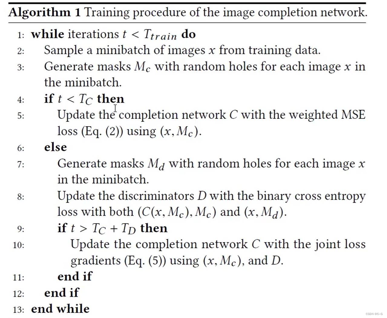
  前Tc次迭代只计算MSE损失，当t大于TC小于Tc+Td时计算判别器损失，当t大于Tc+Td时计算MSE和判别器损失