Opencv Harris corner detection

One 、 Classification of image features

【OpenCV Introduction tutorial 16 】OpenCV Corner detection Harris Corner detection _【 Light ink game programming Blog】 Mao Xingyun （ Light ink ） The column -CSDN Blog _ Corner detection based on contour curve

The following images are from B Station Admiral opencv A screenshot of instructor Jia Zhigang's courseware

1、 edge

2、 Corner point （ Point of interest ）： If a small change of a certain point in any direction will cause a great change in gray level , Then we call it a corner

The corner is located at the intersection of the two edges , Represents the point in the direction of the change of the two edges ,, So they are two-dimensional features that can be accurately located , It can even achieve sub-pixel accuracy , And its image gradient has a high change , This change can be used to help detect corners

3、 speckle （blobs）

Two 、 Corner detection algorithm

thought ：

 Use a fixed window to slide the image in any direction , Compare the two situations before and after sliding , The degree of grayscale change of pixels in the window , If there is sliding in any direction , They all have large gray scale changes , Then we can think of the window as having corners .

In the current field of image processing , Corner detection algorithms can be classified into three categories ：

• Corner detection based on gray image ： Based on the gradient 、 Template based and template based gradient combination
• Corner detection based on binary image ：Harris Corner detection algorithm 、KLT Corner detection algorithm and its application SUSAN Corner detection algorithm
• Corner detection based on contour curve

• There are several specific descriptions of corners ：

  • First derivative ( That is, the gradient of gray ) The pixel corresponding to the local maximum of ;
  • The intersection of two or more edges ;
  • Points in the image where the change rate of gradient value and gradient direction is very high ;
  • The first derivative at the corner is the largest , The second derivative is zero , Indicates the direction in which the edge of an object changes discontinuously .

3、 ... and 、Harris Corner detection principle

From the above, we can know what corner points are , Then let's move the window first , It is described as follows ：

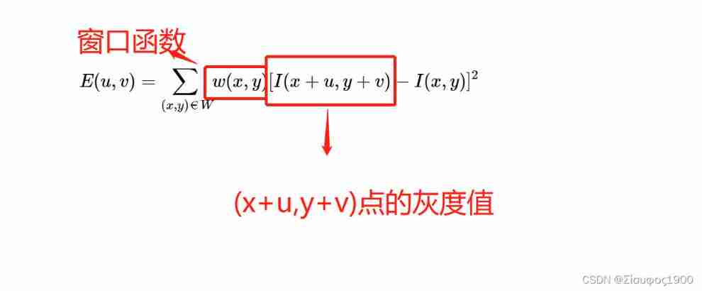
w(x,y) It's a window function , The simplest case is the window W Corresponding to all pixels in w The weight coefficients are 1. But sometimes , We will w(x,y) The function is set to window W Binary positive distribution with the center as the origin . If the window W When the center point is a corner , Before and after moving , This point contributes the most to the gray change ; And leave the window W center ( Corner point ) Far away , The gray changes of these points are almost flat , The weight coefficients of these points , You can set a small value , To show that this point contributes little to the gray change , Then we naturally think of using binary Gaussian function to represent window function .

Then we will review the content of mathematical analysis about Taylor series , Just like any continuous periodic signal can be composed of a set of appropriate sinusoidal curves , Any expression can be approximated infinitely by Taylor formula ：

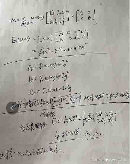
  So let's bring Taylor's formula into the above calculation E（u,v） in ：

  Next is how to solve M This matrix

Are we directly seeking the above E(u,v) Value to judge the corner ？Harris Corner detection does not do this , Instead, you can do this by x The gradient in the direction and y The gradient in the direction is statistically analyzed . Here we use Ix and Iy For the axis , Therefore, the gradient coordinates of each pixel can be expressed as (Ix,Iy). For flat areas , Edge region and corner region are analyzed ：

  Please pay attention to the following picture

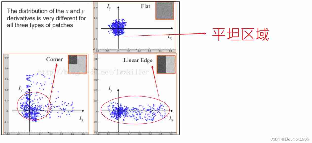
Note the characteristics of these three areas :

• Each pixel on the flat area corresponds to (Ix,Iy) The coordinates are distributed near the origin , It's easy to understand , For pixels in flat areas , Although their gradient directions are different , But its amplitude is not very large , So they all gather near the origin ;
• There is a coordinate axis scattered in the edge area , As for which coordinate the data distribution is scattered, we can't generalize , This depends on the specific position of the edge on the image , If the edge is horizontal or vertical , that Iy Axial direction or Ix The data distribution in the direction is relatively scattered ;
• Corner area x、y The gradient distribution in the direction is relatively scattered .

Can we judge which areas have corners according to these characteristics

 

  Compare the relationship between two eigenvalues ： You can't subtract

 

Conclusion ：

Subtraction is problematic , So how do we use λ1λ2 To express the difference can reflect some of the above conclusions ？

  Define a new function R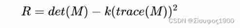  

 det(M)=λ1λ2, determinant

trace(M)=λ1+λ2  trace ;

K Is a comparative value , It is a fixed value we give

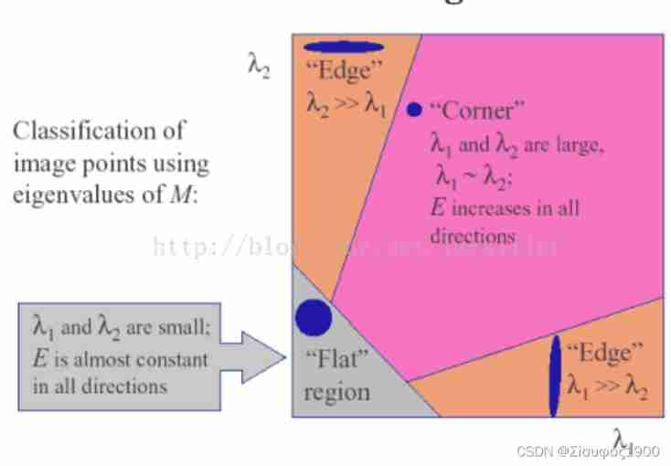
 R Depending on MM The eigenvalues of the ,

For corners |R| It's big ,

Flat areas |R| Very small

Marginal R negative ;

• When the eigenvalues are relatively large , That is, the window contains corners ;
• The eigenvalue is a large one , A smaller one , The window contains edges ;
• The eigenvalues are relatively small , The window is in a flat area ;

Four 、Harris Corner detection steps

1、 Calculate the image x、y Gradient in direction Ix Iy

2、 Calculation Ix* Iy

3、 Use Gaussian function to I2x、I2y、IxIy Gaussian weighting ( take σ=2,ksize=3), The center of calculation is (x,y) The window of WW The corresponding matrix M;

 4、 Calculation R

5、 Filtration is greater than t Of R value  

5、 ... and 、 cornerHarris

void cornerHarris(
 InputArray src, //  It needs to be a single channel 8 Bit or floating point image 
 OutputArray dst,  // Harris Output result of corner detection , The same size and type as the original picture 
 int block Size, // Represents the size of the neighborhood    cornerEigenValsAndVecs() It's said in 
 int ksize,  // Express Sobel() The size of the aperture of the operator 
 double k,  // Calculate k value , Usually take 0.04~0.06;
int borderType = BORDER_DEFAULT // Boundary mode of image pixels . Note that it has a default value BORDER_DEFAULT
)

void cv::cornerHarris( InputArray _src,OutputArray _dst, int blockSize, int ksize, double k, int borderType )
{
   Mat src = _src.getMat();
   _dst.create( src.size(), CV_32F );
   Mat dst = _dst.getMat();
   cornerEigenValsVecs( src, dst, blockSize, ksize, HARRIS, k, borderType);
}

tatic void
cornerEigenValsVecs( const Mat& src,Mat& eigenv, int block_size,
                     int aperture_size, intop_type, double k=0.,
                     intborderType=BORDER_DEFAULT )
{
#ifdef HAVE_TEGRA_OPTIMIZATION
   if (tegra::cornerEigenValsVecs(src, eigenv, block_size, aperture_size,op_type, k, borderType))
       return;
#endif
 
   int depth = src.depth();
   double scale = (double)(1 << ((aperture_size > 0 ?aperture_size : 3) - 1)) * block_size;
   if( aperture_size < 0 )
       scale *= 2.;
   if( depth == CV_8U )
       scale *= 255.;
   scale = 1./scale;
 
   CV_Assert( src.type() == CV_8UC1 || src.type() == CV_32FC1 );
 
   Mat Dx, Dy;
   if( aperture_size > 0 )
    {
       Sobel( src, Dx, CV_32F, 1, 0, aperture_size, scale, 0, borderType );
       Sobel( src, Dy, CV_32F, 0, 1, aperture_size, scale, 0, borderType );
    }
   else
    {
       Scharr( src, Dx, CV_32F, 1, 0, scale, 0, borderType );
       Scharr( src, Dy, CV_32F, 0, 1, scale, 0, borderType );
    }
 
   Size size = src.size();
   Mat cov( size, CV_32FC3 );
   int i, j;
 
   for( i = 0; i < size.height; i++ )
    {
       float* cov_data = (float*)(cov.data + i*cov.step);
       const float* dxdata = (const float*)(Dx.data + i*Dx.step);
       const float* dydata = (const float*)(Dy.data + i*Dy.step);
 
        for( j = 0; j < size.width; j++ )
       {
           float dx = dxdata[j];
           float dy = dydata[j];
 
           cov_data[j*3] = dx*dx;
           cov_data[j*3+1] = dx*dy;
           cov_data[j*3+2] = dy*dy;
       }
    }
 
   boxFilter(cov, cov, cov.depth(), Size(block_size, block_size),
       Point(-1,-1), false, borderType );
 
   if( op_type == MINEIGENVAL )
       calcMinEigenVal( cov, eigenv );
   else if( op_type == HARRIS )
       calcHarris( cov, eigenv, k );
   else if( op_type == EIGENVALSVECS )
       calcEigenValsVecs( cov, eigenv );
}
 
}

6、 ... and 、 Code demonstration

#if  1  // harris   Corner detection 
const  char* INPUT_TITLE = " Original picture ";
const  char* OUT_TITLE = " The original image shows corners ";
const  char* OUT_TITLE2 = " Grayscale image shows corners ";

Mat src, src1, gray;
int g_nThresh = 30; // Current threshold 
int g_nMaxThresh = 175;

void callbackCornerHarris(int, void*)
{
	Mat dstImage; // Goal map 
	Mat normImage; // Normalized graph 
	Mat scaledImage; // The graph of eight bit unsigned shaping after linear transformation 

	//  Set to zero the two pictures currently to be displayed , That is, clear their values the last time this function was called 
	dstImage = Mat::zeros(src.size(), CV_32FC1);
	src1 = src.clone();

	// Corner detection 
	cornerHarris(gray, dstImage, 2, 3, 0.04, BORDER_DEFAULT);
	normalize(dstImage, normImage, 0, 255, NORM_MINMAX, CV_32FC1, Mat());

	// The normalized graph is linearly transformed into 8 Bit unsigned shaping 
	convertScaleAbs(normImage, scaledImage);

	// What will be detected , And the corner points that meet the threshold conditions are drawn 
	for (int i = 0; i < normImage.rows; i++)
	{
		for (int j = 0; j < normImage.cols; j++)
		{
			if ((int)normImage.at<float>(i, j) > g_nThresh + 80)
			{
				circle(src1, Point(j, i), 5, Scalar(10, 10, 255), 2, 8, 0);
				circle(scaledImage, Point(j, i), 5, Scalar(0, 10, 255), 2, 8, 0);
			}
		}
	}
	imshow(OUT_TITLE, src1);
	imshow(OUT_TITLE2, scaledImage);
}

int main()
{
	src = imread("C:\\Users\\19473\\Desktop\\opencv_images\\corners.png");
	if (!src.data)
	{
		printf("could not  load  image....\n");
	}
	imshow(INPUT_TITLE, src);
	src.copyTo(src1);
	cvtColor(src1, gray, COLOR_BGR2GRAY);

	namedWindow(OUT_TITLE, WINDOW_AUTOSIZE);
	createTrackbar(" threshold ：", OUT_TITLE, &g_nThresh, g_nMaxThresh, callbackCornerHarris);

	callbackCornerHarris(0, NULL);

	waitKey(0);
	return 0;
}

#endif