1. Introduction to generating countermeasures network

GAN brief introduction （Generative Adversarial Nets）

Thief （Generator Network） Through random variables （Random Vector） Generate fake money （Fake Image） Deposit into bank （Discriminator Network）, Banks use real money （Real Image）、 Fake money （Fake Image） Learn to judge the fake money of thieves , Cycle the above steps .

The thief wanted the bank to judge the fake money as real money , So fake money （ Tag value is true ） Leave it to the bank for judgment , Get feedback from the bank loss, This is used for update iterations , Optimize counterfeiting technology

The bank hopes to accurately judge the real and counterfeit money , So at the same time, the thief's fake money （ Tag value is false ）、 And real money for training （ Tag value is true ） Training , This is used for update iterations

Loss function

import torch
from torch import autograd
import torch.nn as nn
import math

input = autograd.Variable(torch.tensor([
    [1.9072, 1.1079, 1.4906],
    [-0.6548, -0.0512, 0.7608],
    [-0.0614, 0.6583, 0.1095]
]))
print(input)
print('-' * 100)

m = nn.Sigmoid()
print(m(input))
print('-' * 100)

target = torch.FloatTensor([
    [0, 1, 1],
    [1, 1, 1],
    [0, 0, 0]
])
print(target)
print('-' * 100)

r11 = 0 * math.log(0.8707) + (1 - 0) * math.log((1 - 0.8707))
r12 = 1 * math.log(0.7517) + (1 - 1) * math.log((1 - 0.7517))
r13 = 1 * math.log(0.8162) + (1 - 1) * math.log((1 - 0.8162))

r21 = 1 * math.log(0.3419) + (1 - 1) * math.log((1 - 0.3419))
r22 = 1 * math.log(0.4872) + (1 - 1) * math.log((1 - 0.4872))
r23 = 1 * math.log(0.6815) + (1 - 1) * math.log((1 - 0.6815))

r31 = 0 * math.log(0.4847) + (1 - 0) * math.log((1 - 0.4847))
r32 = 0 * math.log(0.6589) + (1 - 0) * math.log((1 - 0.6589))
r33 = 0 * math.log(0.5273) + (1 - 0) * math.log((1 - 0.5273))

r1 = -(r11 + r12 + r13) / 3
r2 = -(r21 + r22 + r23) / 3
r3 = -(r31 + r32 + r33) / 3

bceloss = (r1 + r2 + r3) / 3
print(bceloss)
print('-' * 100)


# torch  need Sigmoid
loss = nn.BCELoss()
print(loss(m(input), target))
print('-' * 100)

# torch  Unwanted Sigmoid
loss = nn.BCEWithLogitsLoss()
print(loss(input, target))
print('-' * 100)

CycleGan

brief introduction

• Realization effect

• No pairing data is required

• How to learn
  
  generator Gab Make a fake horse from a real zebra , Fake horse passing Gba Generate fake zebras , False zebra and real zebra produce L2 Loss , Iterative optimization

• Overall network architecture
  

• PatchGAN
  

Entry test

• Source code address

https://github.com/junyanz/pytorch-CycleGAN-and-pix2pix

• Data download
  Open the file as text
  
  Copy download link
  
  
• Trained parameter weights
  

https://github.com/junyanz/pytorch-CycleGAN-and-pix2pix/blob/master/scripts/download_cyclegan_model.sh#L3

http://efrosgans.eecs.berkeley.edu/cyclegan/pretrained_models/

Will download okay horse2zebra.pth Files in pytorch-CycleGAN-and-pix2pix-master\checkpoints\horse2zebra_pretrained Next , And change the name to latest_net_G.pth

• Start the test

Test parameters

--dataroot datasets/horse2zebra/testA
--name horse2zebra.pth_pretrained
--model test --no_dropout
#  Use cpu
--gpu_ids -1

stay pytorch-CycleGAN-and-pix2pix-master\results\horse2zebra_pretrained\test_latest Save the results under

open index.html

visdom

CycleGan Use during training visdom As a visualization tool , Start before training visdom

pip install visdom
python -m visdom.server

stargan

• What is the star

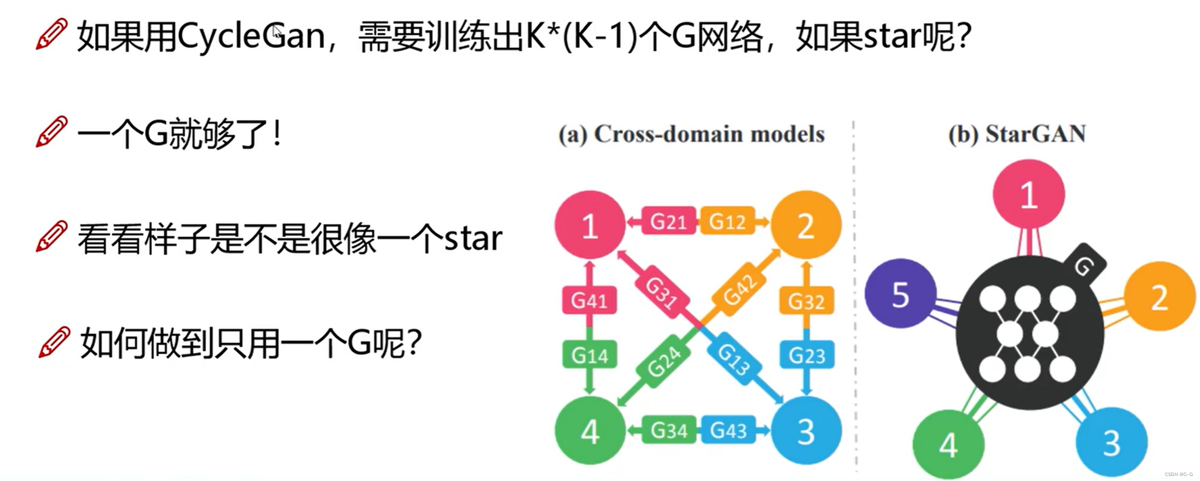
• The basic idea
  
• Overall process
  
  
  Input picture and coding features , Get fake photos through the generator , Then the fake photos are generated to get the real photos , And compare with the original drawing , Narrow the gap between the real photos and the original pictures

stargan Use coding instead of style , Not very characteristic , Not involved in the calculation

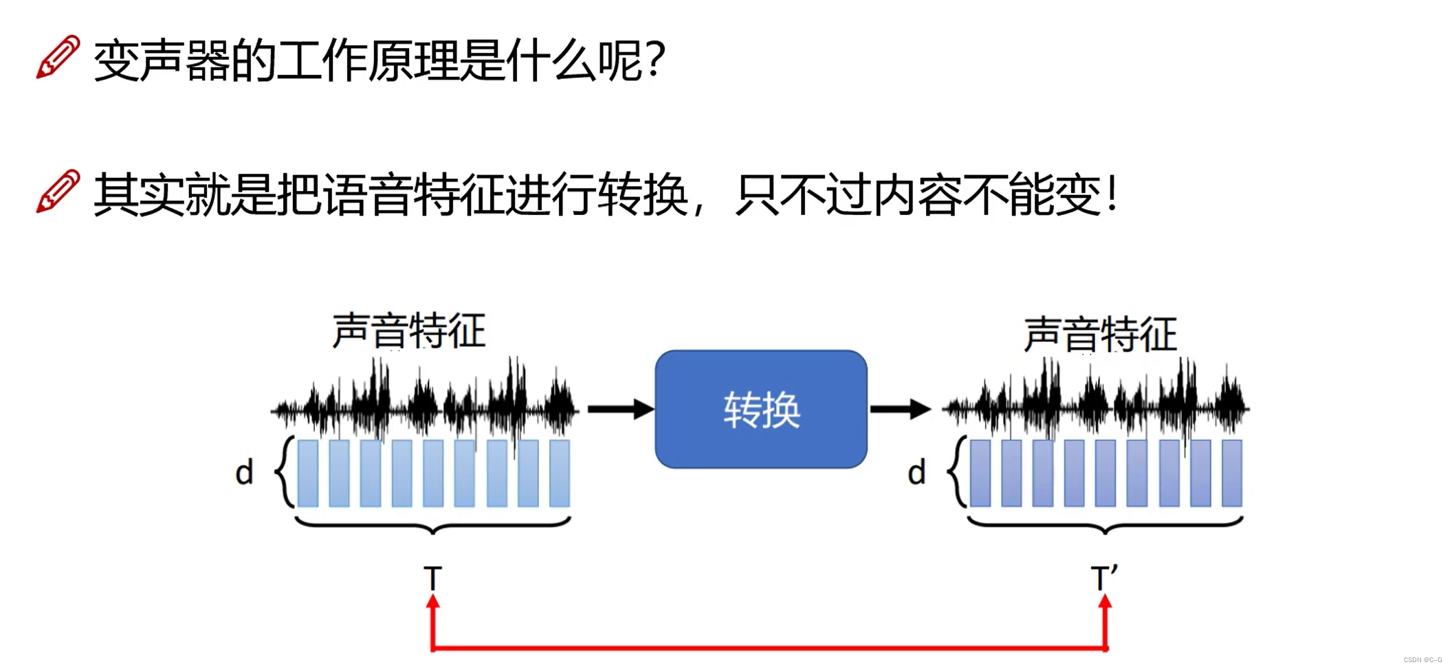
• Expand ： Sound transformer
  

stargan-v2

• Overall network architecture
  
• Encoder training （Style reconstruction）

• Diversified training （Style diversification）
  
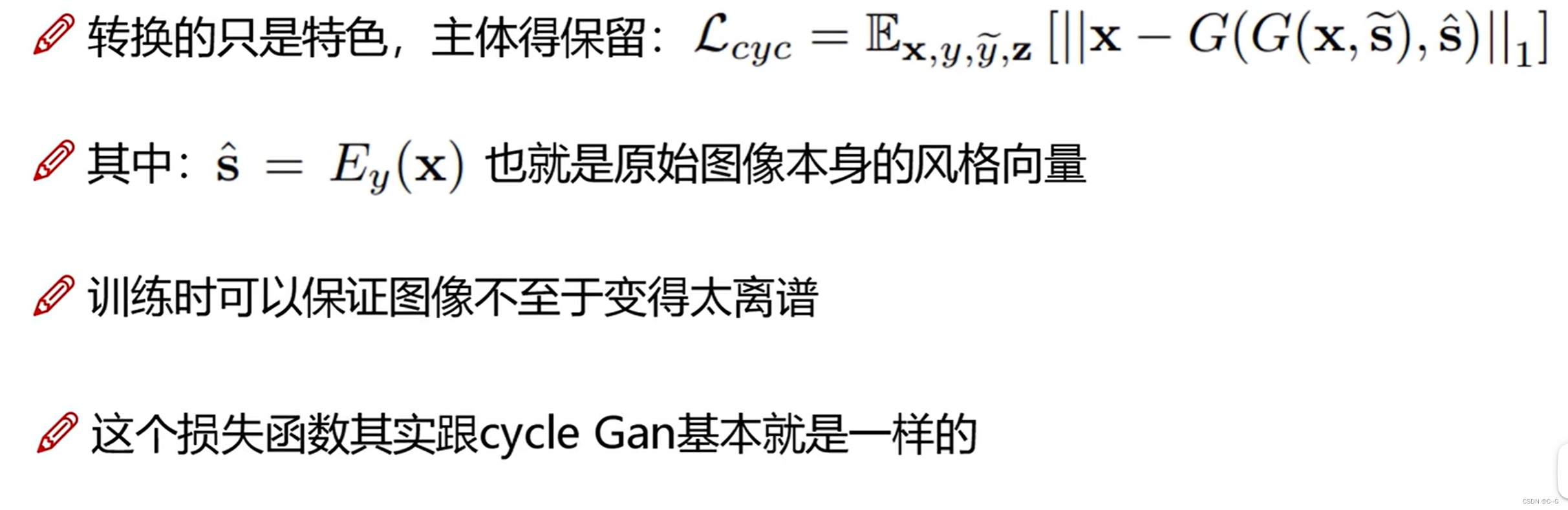
• cycle loss

The code analysis

• Source download
  https://github.com/clovaai/stargan-v2
• Import the necessary packages

conda create -n stargan-v2 python=3.6.7
conda activate stargan-v2
conda install -y pytorch=1.4.0 torchvision=0.5.0 cudatoolkit=10.0 -c pytorch
conda install x264=='1!152.20180717' ffmpeg=4.0.2 -c conda-forge
pip install opencv-python==4.1.2.30 ffmpeg-python==0.2.0 scikit-image==0.16.2
pip install pillow==7.0.0 scipy==1.2.1 tqdm==4.43.0 munch==2.5.0

• generator

class Generator(nn.Module):
    def __init__(self, img_size=256, style_dim=64, max_conv_dim=512, w_hpf=1):
        super().__init__()
        dim_in = 2**14 // img_size
        self.img_size = img_size
        self.from_rgb = nn.Conv2d(3, dim_in, 3, 1, 1)
        self.encode = nn.ModuleList()
        self.decode = nn.ModuleList()
        self.to_rgb = nn.Sequential(
            nn.InstanceNorm2d(dim_in, affine=True),
            nn.LeakyReLU(0.2),
            nn.Conv2d(dim_in, 3, 1, 1, 0))

        # down/up-sampling blocks
        repeat_num = int(np.log2(img_size)) - 4
        if w_hpf > 0:
            repeat_num += 1
        for _ in range(repeat_num):
            dim_out = min(dim_in*2, max_conv_dim)
            self.encode.append(
                ResBlk(dim_in, dim_out, normalize=True, downsample=True))
            self.decode.insert(
                0, AdainResBlk(dim_out, dim_in, style_dim,
                               w_hpf=w_hpf, upsample=True))  # stack-like
            dim_in = dim_out

        # bottleneck blocks
        for _ in range(2):
            self.encode.append(
                ResBlk(dim_out, dim_out, normalize=True))
            self.decode.insert(
                0, AdainResBlk(dim_out, dim_out, style_dim, w_hpf=w_hpf))

        if w_hpf > 0:
            device = torch.device(
                'cuda' if torch.cuda.is_available() else 'cpu')
            self.hpf = HighPass(w_hpf, device)

    def forward(self, x, s, masks=None):
        x = self.from_rgb(x)
        cache = {
    }
        for block in self.encode:
            if (masks is not None) and (x.size(2) in [32, 64, 128]):
                cache[x.size(2)] = x
            x = block(x)
        for block in self.decode:
            x = block(x, s)
            if (masks is not None) and (x.size(2) in [32, 64, 128]):
                mask = masks[0] if x.size(2) in [32] else masks[1]
                mask = F.interpolate(mask, size=x.size(2), mode='bilinear')
                x = x + self.hpf(mask * cache[x.size(2)])
        return self.to_rgb(x)

Normalized layer , At present, there are mainly these methods ,Batch Normalization（2015 year ）、Layer Normalization（2016 year ）、Instance Normalization（2017 year ）、Group Normalization（2018 year ）、Switchable Normalization（2018 year ）;

Will input the image shape Write it down as [N, C, H, W], The main difference between these methods is ,

• batchNorm Is in batch On , Yes NHW Normalization , Yes, small batchsize The result is bad ;
• layerNorm In the direction of the passage , Yes CHW normalization , Mainly for RNN The effect is obvious ;
• instanceNorm On the image pixels , Yes HW Normalization , Used in stylized migration ;
• GroupNorm take channel grouping , And then do normalization ;
• SwitchableNorm Yes, it will BN、LN、IN combination , Give weight to , Let the network learn the normalization layer by itself .

• Style feature code

class MappingNetwork(nn.Module):
    def __init__(self, latent_dim=16, style_dim=64, num_domains=2):
        super().__init__()
        layers = []
        layers += [nn.Linear(latent_dim, 512)]
        layers += [nn.ReLU()]
        for _ in range(3):
            layers += [nn.Linear(512, 512)]
            layers += [nn.ReLU()]
        self.shared = nn.Sequential(*layers)

        self.unshared = nn.ModuleList()
        for _ in range(num_domains):
            self.unshared += [nn.Sequential(nn.Linear(512, 512),
                                            nn.ReLU(),
                                            nn.Linear(512, 512),
                                            nn.ReLU(),
                                            nn.Linear(512, 512),
                                            nn.ReLU(),
                                            nn.Linear(512, style_dim))]

    def forward(self, z, y):
        h = self.shared(z)
        out = []
        for layer in self.unshared:
            out += [layer(h)]
        out = torch.stack(out, dim=1)  # (batch, num_domains, style_dim)
        idx = torch.LongTensor(range(y.size(0))).to(y.device)
        s = out[idx, y]  # (batch, style_dim)
        return s

• Judging device

class Discriminator(nn.Module):
    def __init__(self, img_size=256, num_domains=2, max_conv_dim=512):
        super().__init__()
        dim_in = 2**14 // img_size
        blocks = []
        blocks += [nn.Conv2d(3, dim_in, 3, 1, 1)]

        repeat_num = int(np.log2(img_size)) - 2
        for _ in range(repeat_num):
            dim_out = min(dim_in*2, max_conv_dim)
            blocks += [ResBlk(dim_in, dim_out, downsample=True)]
            dim_in = dim_out

        blocks += [nn.LeakyReLU(0.2)]
        blocks += [nn.Conv2d(dim_out, dim_out, 4, 1, 0)]
        blocks += [nn.LeakyReLU(0.2)]
        blocks += [nn.Conv2d(dim_out, num_domains, 1, 1, 0)]
        self.main = nn.Sequential(*blocks)

    def forward(self, x, y):
        out = self.main(x)
        out = out.view(out.size(0), -1)  # (batch, num_domains)
        idx = torch.LongTensor(range(y.size(0))).to(y.device)
        out = out[idx, y]  # (batch)
        return out

stargan-vc2

http://www.kecl.ntt.co.jp/people/kaneko.takuhiro/projects/stargan-vc2/index.html

• Sound transformer

• input data
  

• Preprocessing
  

• Feature summary
  

• MFCC
  

• generator
  

• The components contained in linguistic data
  

• Instance Normalization and Adaptive Instance Normalization
  

• Instance Normalization
  
  The content encoder only needs content , No linguistic features are required , So use Instance Normalization Normalize each feature map , Average the sound characteristics , Remove language features

• AdaIn
  
  In Normalization removes linguistic features ,AdaIn Through additional FC Layers give language features

• PixelShuffle
  Up sampling and down sampling ： They are all old ways ,stride=2 Let's take a sample , Deconvolution to upsample
  **PixelShuffle Layer is also known as sub-pixel convolution layer , It's a paper Real-Time Single Image and Video Super-Resolution Using an Efficient Sub-Pixel Convolutional Neural Network A convolution layer with up sampling function for super-resolution reconstruction is introduced in . This article ESPCN This paper introduces the function of this layer ,sub-pixel convolution layer With stride = 1 r stride=\frac{1}{r}stride= r1 (r rr by SR The magnification of upscaling factor) To extract feature map, Although it is called convolution , But it doesn't use any parameters that need to be learned , Its principle is very simple , Is to enter feature map Pixel reorganization , In other words, although the sub-pixel convolution layer is called convolution , But I didn't do any multiplication and addition , It's just another way to extract features ：
  **

The last layer shown above is the sub-pixel convolution layer , It is to format the input as ( b a t c h , r 2 C , H , W ) (batch,r^2C, H, W)(batch,r 2C,H,W) Of feature map The pixels in the same channel are extracted as output feature map A small piece of , Traverse the entire input feature map You can get the final output image . On the whole , It's like using 1r\frac{1}{r}r1 The step size is the same as convolution , This results in not convoluting the whole pixel , It's convolution of subpixels , Therefore, it is called sub-pixel convolution layer , The final output format is ( b a t c h , 1 , r H , r W ) (batch,1, rH,rW)(batch,1,rH,rW).

therefore , In a word ,PixelShuffle What the layer does is input feature map Pixel reorganization outputs high-resolution images feature map, Is an up sampling method , The specific expression is

among r Is the upper sampling magnification ( Above picture r = 3)

• Judging device
  

Image super-resolution reconstruction （SPGAN）

• Network architecture

• The basic idea

Basic GAN Network thinking , The generator uses PixelShuffle Achieve super-resolution reconstruction , At the same time, in order to improve the detail effect , introduce vgg19, Put the false and true graphs generated by the generator into vgg19 Model extraction features , And extract the last layer of characteristic graph to calculate the loss , Add this loss to the generator loss

• Tools

tensorlayer

Image completion

The paper ：Globally and Locally Consistent Image Completion

• Network architecture
  

• Fully convolutional network , Do not limit the size of the input picture

• Dilated Conv Cavity convolution Increase the receptive field replace pooling

• Local Discriminator Local discriminant network Collect local information
  

• Global Discriminator Global discriminant network Collect global information
  

• Image generation network
  

• The final synthetic network
  

• MSE Loss
  
  By generating the image and the original MSE Loss , Avoid over relying on the feature judgment of the discriminator

• Calculate the loss step by step
  
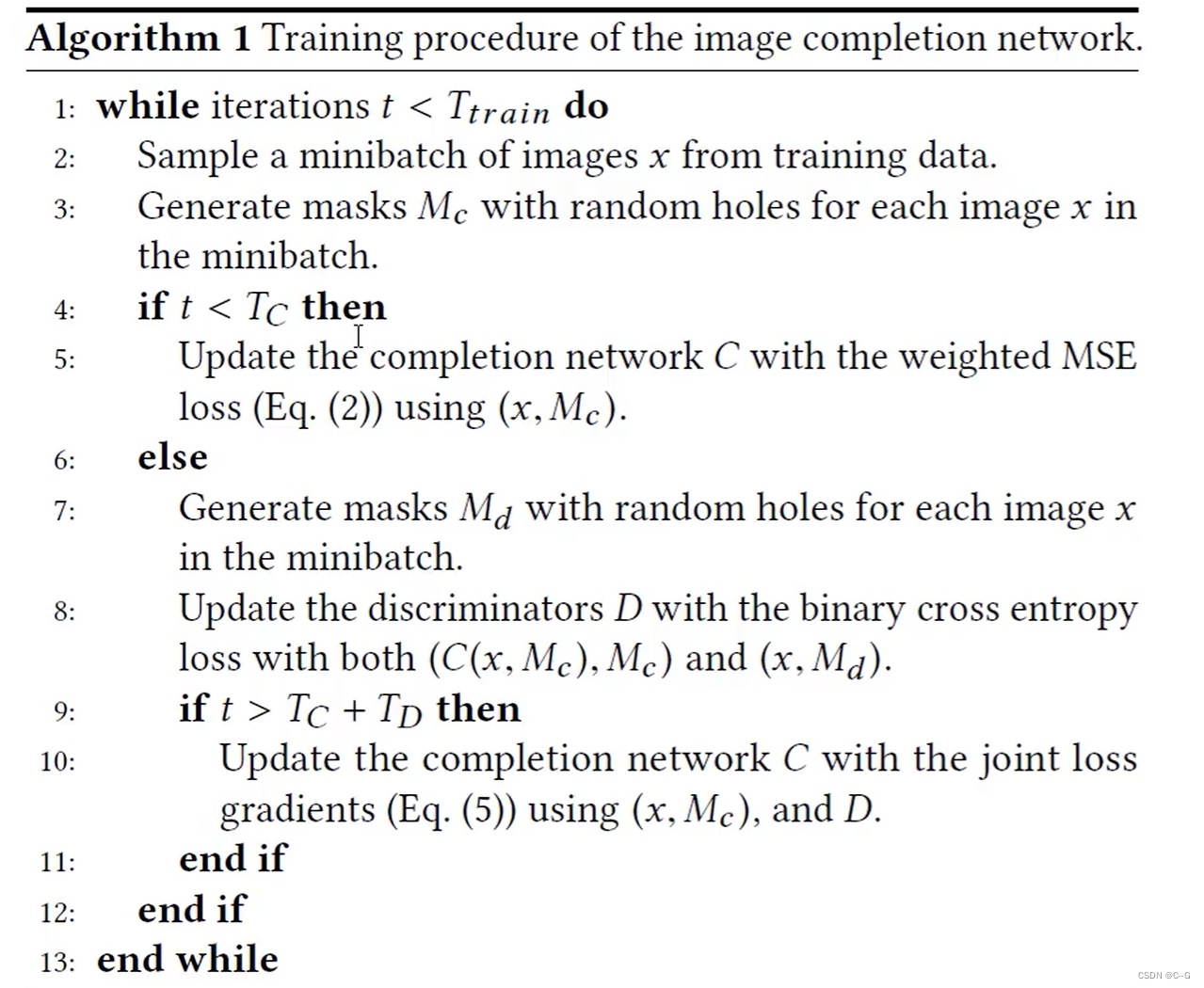
  front Tc Calculation only in the next iteration MSE Loss , When t Greater than TC Less than Tc+Td Calculate the discriminator loss , When t Greater than Tc+Td Hourly calculation MSE And discriminator loss