当前位置:网站首页>Gaussian filtering and bilateral filtering principle, matlab implementation and result comparison
Gaussian filtering and bilateral filtering principle, matlab implementation and result comparison
2022-07-08 02:15:00 【Strawberry sauce toast】
This paper introduces the principles of Gaussian filtering and bilateral filtering in detail and gives MATLAB Realization , Finally, compare the effect of Gaussian filtering and bilateral filtering .
Catalog
1.1 One dimensional Gaussian distribution
1.2 Two dimensional Gaussian distribution
1.3 Gaussian filtering summary
1. The principle of bilateral filtering
2. How to realize bilateral filtering “ Edge preserving denoising ” Of ?
3. MATLAB Realize bilateral filtering
4. About sigma Value selection
4.1 Space domain sigma selection
3、 ... and 、 The results of bilateral filtering and Gaussian filtering are compared
3.1 Simulation image comparison
One 、 Filtering principle
Reference resources :https://blog.csdn.net/nima1994/article/details/79776802( The principle of Gaussian filtering )
Focus on :
The essence of spatial filtering is in the window “ Take the average ”, The larger the radius of the template , The stronger the blur effect .
Gaussian filtering , Gaussian function is used to calculate the template weight , It is based on : In continuous images , The closer the point is, the closer the relationship is , The farther away the point, the more distant the relationship , therefore , The weighted average is more reasonable , That is, the closer to the center point, the greater the weight of the point , The farther the distance, the smaller the weight of the point .
1.1 One dimensional Gaussian distribution
One dimensional Gaussian distribution ( Normal distribution ) Just meet this condition , Pictured 1.

chart 1 Normal distribution “ A bell curve ”
One dimensional Gaussian distribution formula is shown in formula (1), The mean is  Determines the center point of the curve ,
 Determines the width of the curve , The larger the curve, the wider .
 …………(1)
MATLAB Realize one-dimensional Gaussian function :
function g = Gaussian(X,avg,sigma)
%%  Functional specifications : One dimensional Gaussian distribution
%%  Parameter description :avg --  mean value , Determine the location of the center point
%          sigma --  Standard deviation , Determine the curve width
   temp_1 = 1 / (sigma * sqrt(2*pi));
   temp_2 = -(X - avg).^2./(2*sigma^2);
   g = temp_1 * exp(temp_2);
   g = g ./ sum(g(:));
end
Use the above functions to draw different Value corresponds to the curve , The code is as follows :
X = -15:0.1:15;
avg = 0;  %  The center point of the image is 0
sigmas = [1;2;3;4];
for i = 1:length(sigmas)
    g = Gaussian(X,avg,sigmas(i));
    plot(X,g)
    hold on
end
legend('\sigma = 1','\sigma = 2','\sigma = 3','\sigma = 4');
The image is like this 2, obviously , Determines the width of the curve , The larger the curve, the wider , And the image is about x = avg( Here for 0) symmetry .

chart 2 Different Value corresponding to one-dimensional Gaussian distribution
Additional explanation : I did before min-max Standardization , Will be different sigma The value range of the curve corresponding to the value is mapped in [0,1] Within the scope of , But now I find that this practice ignores sigma Influence of value on curve height .
( Properties of Gaussian distribution : Below the curve and x The sum of the areas above the shaft is 1)sigma The value of not only determines the width of the curve , It also determines the height of the curve ,sigma The bigger it is , The wider the curve, the shorter ;sigma The smaller it is , The narrower the curve, the higher .
1.2 Two dimensional Gaussian distribution
take x = x,y Substitute into the formula (1) after , Two dimensional Gaussian distribution formula can be obtained by multiplying the two (2):
 …………(2)
Here is the order A simplified two-dimensional Gaussian distribution function formula can be obtained (3):
 …………(3)
According to the formula (3) You can calculate the weight of each point in the Gaussian filter template .
Two dimensional Gaussian function , The code is as follows :
function [G] = Gaussian(R,sigma)
%%  Functional specifications : Two dimensional Gaussian function , It can be used to calculate the Gaussian filter weight matrix
%           Gauss filtering : Only airspace information is considered , Gray similarity is not considered
%%  Input parameters :R --  Formwork radius
%          sigma --  Standard deviation
    [X,Y] = meshgrid(-R:0.1:R);
    temp1 = 1/(2*pi*sigma^2);
    temp2 = -(X.^2 + Y.^2)/(2*sigma^2);
    G = temp1 * exp(temp2);

    G = G./sum(G(:));  %  The sum of the weights of the template must be equal to 1.

    %  Draw a template diagram
    figure
    surf(X,Y,G);
    shading interp;
end
The size is 15*15, The standard deviation is 2 The two-dimensional Gaussian distribution template of is shown in the figure 3 Shown

chart 3 The size is 11*11 Two dimensional Gaussian distribution
Use a size of 5*5, The standard deviation is 0.3 Gaussian blur is applied to the image containing weak targets and clouds , Pictured 4 Shown .

chart 4 The size is 5*5, The standard deviation is 0.3 Template Gaussian fuzzy filtering results
1.3 Gaussian filtering summary
Gaussian filtering only considers the spatial similarity between image pixels , That is, in continuous images , The closer the point is, the closer the relationship is , The farther away the point, the more distant the relationship .
Two 、 Bilateral filtering
1. The principle of bilateral filtering
Reference resources :https://blog.csdn.net/Chaolei3/article/details/88579377
Bilateral filtering is a nonlinear method , Compared with Gaussian filtering , Bilateral filtering not only considers the spatial similarity of images , The gray similarity is also considered , You can achieve “ Edge preserving denoising ” Purpose .
Bilateral filtering consists of two parts : Spatial matrix and range matrix , Spatial matrix can be analogous to Gaussian filtering , Used for blur denoising ; The range matrix is obtained according to the gray similarity , Used to protect edges .
Calculation formula of spatial matrix (4), Range matrix calculation formula (5)
 …………(4)
 …………(5)
Formula description : Definition (i, j) Is the coordinate of the center point ,(k, l) For the point (i, j) Is any point in the neighborhood of the center .
The formula (4)(5) Multiplication is the calculation formula of bilateral filter weight matrix (6)
 …………(6)
Last , Calculate the weighted average value as the filtered value of the central point coordinate
 ………… (7)
2. How to realize bilateral filtering “ Edge preserving denoising ” Of ?
By formula (4), The weight distribution of the spatial domain weight matrix is still “ Bell shape ”, That is, the closer to the center , The greater the weight ;
By formula (5)(6), It is known that  Yes (0,1) The subtraction function of points , That is, the greater the gray difference , The less weight , The worse the smoothing effect , conversely , The smaller the gray difference , The greater the weight , The better the smoothing effect . therefore , When the center point is at the edge , Large gray difference , The spatial domain smoothing effect is weakened , The edges are preserved ; When the neighborhood gray value is close to the center point , The gray difference is close to 0, The weight of the range is close to 1, At this time, the filtering effect depends on the spatial domain weight matrix , The effect is consistent with Gaussian filtering .
The formula (7) The meaning of : The value of the center point after filtering = Weight matrices .* original image ( And ensure that the sum of weights is 1, normalization )( Refer to the filtering principle )

chart 5 Bilateral filtering “ Edge preserving denoising ” Schematic diagram
3. MATLAB Realize bilateral filtering
function b = BF_Filter(img,r,sigma_d,sigma_r)
%%  Functional specifications : Bilateral filtering , Used to calculate the image after bilateral filtering
%           Bilateral filtering is a nonlinear method , At the same time, the spatial information and gray similarity of the image are considered .
%           A new weight matrix is formed by spatial matrix and range matrix , among , Spatial matrix is used for fuzzy denoising , The range matrix is used to protect the edge .
%%  Input parameters :img --  Image to be filtered
%          r --  Formwork radius ,e.g. 3*3 The radius of the template is 1
%          sigma_d --  Standard deviation of spatial matrix
%          sigma_r --  Range matrix standard deviation

    %  Determine whether it is a grayscale image
    if(size(img,3)>1)
        img = rgb2gray(img);
    end
    [x,y] = meshgrid(-r:r);

    %  Airspace weight matrix  size = (2r+1)*(2r+1)
    w_spacial = exp(-(x.^2 + y.^2)/(2*sigma_d.^2));

    [m,n] = size(img);
    img = double(img);

    %  Expand the image ,size = (m+2r)*(n+2r)
    f_temp = padarray(img,[r r],'symmetric');

    %  Slide the window and filter
    b = zeros(m,n); %  The filtered image
    for i = r+1:m+r
        for j = r+1:n+r
            temp = f_temp(i-r:i+r,j-r:j+r);
            w_value = exp(-(temp - img(i-r,j-r)).^2/(2*sigma_r^2));  % size = (2r+1)*(2r+1)
            w = w_spacial .* w_value;
            s = temp.*w;
            b(i-r,j-r) = sum(s(:))/sum(w(:));
        end
    end
end
4. About sigma Value selection
4.1 Space domain sigma  selection
The size of the nucleus is usually , namely

Because it is far from the center The coefficient outside the size is smaller than the coefficient at the midpoint , It can be considered that the other points have little connection with the central point , The weight coefficient can be regarded as 0.
4.2 range sigma  selection

chart 6 Images
When  , The range of gray difference is [0,255] when ,x Value range of
  , The range of values is :[0.3679,1];
When  , The range of gray difference is [0,255] when ,x Value range of
  , The range of values is :[0.01832,1];
therefore ,sigma The bigger it is , The smaller the range of weight value , At this time, even if the difference between the neighborhood gray value and the center point gray value is large , Its corresponding weight will also be large , This is related to bilateral filtering “ Edge preserving ” Against the original intention of ;sigma The smaller it is , The larger the range of weight value , At this time, when the difference between the gray values of the center point of the neighborhood gray value range is large , The smaller the corresponding weight , Can weaken “ smooth ”, achieve “ Edge preserving ” effect .
Sum up ,sigma The bigger it is , The more blurred the edge ,sigma-->∞ when ,x-->0, The weight -->1, Multiplied by Gaussian template, it can be considered as equivalent to Gaussian filtering ;
sigma The smaller it is , The clearer the edge ,sigma-->0 when ,x-->∞, The weight -->0, When multiplied by Gaussian template, the coefficients are all equal , Equivalent to the source image .
3、 ... and 、 The results of bilateral filtering and Gaussian filtering are compared
3.1 Simulation image comparison
Generate an image with obvious edges , Pictured 7 Shown .

chart 7 Simulation image
img_B = zeros(250,250);
img_B(:,40:50) = 1;
img_B(:,180:200) = 1;
img_B(100:105,:) = 1;
imshow(img_B)
The results of Gaussian filtering and bilateral filtering are shown in the figure 8 Shown , obviously , Bilateral filtering can better preserve the edge information of the image .

chart 8 Comparison results of simulation images of bilateral filtering and Gaussian filtering
%%  Gauss filtering
r = 7;
sigma_d = 1;
G = Gaussian(r, sigma_d);
g = imfilter(img_B, G, 'symmetric');
%%  Bilateral filtering
sigma_r = 3;
b = BF_Filter(img_B,r,sigma_d,sigma_r);
figure
subplot(1,2,1)
imshow(b);title([num2str(2*r+1),'*',num2str(2*r+1),' Bilateral filtering results ','\sigma_d=1 ,',' \sigma_r=3']);
subplot(1,2,2)
imshow(g);title([num2str(2*r+1),'*',num2str(2*r+1),' Gaussian filtering result ','\sigma_d=1']);
3.2 Real image comparison
From the results , For images with structural backgrounds such as clouds and weak targets , Compared with Gaussian filtering , Bilateral filtering can well preserve the edge of the image ( structure ) Information .

chart 9 Original real image

chart 10 Comparison results of real images with bilateral filtering and Gaussian filtering
img = imread('cloud.bmp');
if(size(img,3)>1)
    img = rgb2gray(img);
end
r = 7;
sigma_d = 0.5;
G = Gaussian(r, sigma_d);
img_g = imfilter(img, G, 'symmetric');

sigma_r = 3;
img_b = BF_Filter(img,r,sigma_d,sigma_r);
subplot(1,3,1);
imshow(img);title(' Original picture ');
subplot(1,3,2)
imshow(img_g,[]);title(' Gaussian filtering result ');
subplot(1,3,3);
imshow(img_b,[]);title(' Bilateral filtering results ');
3.3 summary
Combined with the subject of weak and small target detection , Bilateral filtering is suitable for predicting rich edges ( structure ) Background prediction of information , Choose the right one through experiments sigma value , Predict the background , Original picture - Forecast background = Goal map (STI), And then from STI Detect the target in the figure , The next step needs to be explored .
边栏推荐
- I don't know. The real interest rate of Huabai installment is so high
- Random walk reasoning and learning in large-scale knowledge base
- Nanny level tutorial: Azkaban executes jar package (with test samples and results)
- Xmeter newsletter 2022-06 enterprise v3.2.3 release, error log and test report chart optimization
- 咋吃都不胖的朋友,Nature告诉你原因:是基因突变了
- Principle of least square method and matlab code implementation
- Little knowledge about TXE and TC flag bits
- LeetCode精选200道--链表篇
- 2022国内十大工业级三维视觉引导企业一览
- [knowledge map] interpretable recommendation based on knowledge map through deep reinforcement learning
猜你喜欢

Applet running under the framework of fluent 3.0

进程和线程的退出

ClickHouse原理解析与应用实践》读书笔记(8)

Completion report of communication software development and Application
Matlab r2021b installing libsvm

Alo who likes TestMan
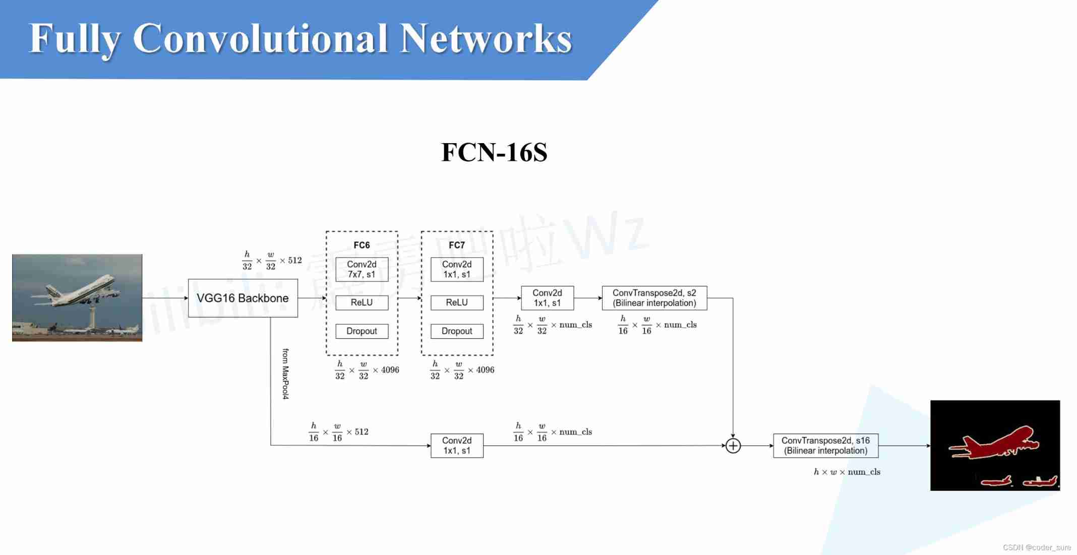
Semantic segmentation | learning record (3) FCN
Talk about the realization of authority control and transaction record function of SAP system

Disk rust -- add a log to the program

数据链路层及网络层协议要点
随机推荐
XMeter Newsletter 2022-06|企业版 v3.2.3 发布,错误日志与测试报告图表优化
JVM memory and garbage collection-3-runtime data area / heap area
VIM string substitution
2022年5月互联网医疗领域月度观察
burpsuite
[knowledge map paper] r2d2: knowledge map reasoning based on debate dynamics
Matlab r2021b installing libsvm
Leetcode question brushing record | 485_ Maximum number of consecutive ones
[target tracking] |atom
直接加比较合适
Introduction to grpc for cloud native application development
Towards an endless language learning framework
很多小伙伴不太了解ORM框架的底层原理,这不,冰河带你10分钟手撸一个极简版ORM框架(赶快收藏吧)
[knowledge atlas paper] minerva: use reinforcement learning to infer paths in the knowledge base
metasploit
Strive to ensure that domestic events should be held as much as possible, and the State General Administration of sports has made it clear that offline sports events should be resumed safely and order
List of top ten domestic industrial 3D visual guidance enterprises in 2022
burpsuite
What are the types of system tests? Let me introduce them to you
Clickhouse principle analysis and application practice "reading notes (8)