当前位置:网站首页>Ml self realization / logistic regression / binary classification
Ml self realization / logistic regression / binary classification
2022-07-08 01:58:00 【xcrj】
principle
Prediction function :
- classification : 0 ≤ h θ ( x ) ≤ 1 0\leq h_\theta(x)\leq1 0≤hθ(x)≤1
- Tradition : h θ ( x ) ≫ 1 ∣ ∣ h θ ( x ) ≪ 0 h_\theta(x)\gg 1 || h_\theta(x)\ll 0 hθ(x)≫1∣∣hθ(x)≪0
Traditional prediction function is transformed into classification prediction function :
- Traditional prediction function h θ ( x ) h_\theta(x) hθ(x) * s i g m o i d \stackrel{sigmoid}{\longrightarrow} *sigmoid Classification prediction function h θ ( x ) h_\theta(x) hθ(x)

The process :
sigmoid: g ( z ) = 1 1 + e − z * z = h θ ( x ) = θ T x = 1 1 + e − θ T x g(z)=\frac{1}{1+e^{-z}}\stackrel{z=h_\theta(x)=\theta^Tx}{\longrightarrow}=\frac{1}{1+e^{-\theta^Tx}} g(z)=1+e−z1*z=hθ(x)=θTx=1+e−θTx1
primary h θ ( x ) = z = θ T x = θ 0 + θ 1 x 1 + θ 2 x 2 + . . . + θ n x n h_\theta(x)=z=\theta^Tx=\theta_0+\theta_1x_1+\theta_2x_2+...+\theta_nx_n hθ(x)=z=θTx=θ0+θ1x1+θ2x2+...+θnxn
new h θ ( x ) = P ( y = 1 ∣ x ; θ ) = 1 1 + e − z h_\theta(x)=P(y=1|x;\theta)=\frac{1}{1+e^{-z}} hθ(x)=P(y=1∣x;θ)=1+e−z1
Decision boundaries :
- new h θ ( x ) = g ( z ) ≥ 0.5 when , recognize by y = 1 ⇒ z ≥ 0 ⇒ θ T x ≥ 0 ⇒ used h θ ( x ) ≥ 0 new h_\theta(x)=g(z) \geq0.5 when , Think y=1 \Rightarrow z \geq0 \Rightarrow \theta^Tx \geq0 \Rightarrow used h_\theta(x) \geq0 new hθ(x)=g(z)≥0.5 when , recognize by y=1⇒z≥0⇒θTx≥0⇒ used hθ(x)≥0
- new h θ ( x ) = g ( z ) ≤ 0.5 when , recognize by y = 0 ⇒ z ≤ 0 ⇒ θ T x ≤ 0 ⇒ used h θ ( x ) ≤ 0 new h_\theta(x)=g(z) \leq0.5 when , Think y=0 \Rightarrow z \leq0 \Rightarrow \theta^Tx \leq0 \Rightarrow used h_\theta(x) \leq0 new hθ(x)=g(z)≤0.5 when , recognize by y=0⇒z≤0⇒θTx≤0⇒ used hθ(x)≤0
- used h θ ( x ) = 0 , Just yes " Strategy edge world used h_\theta(x)=0, It's the decision boundary used hθ(x)=0, Just yes " Strategy edge world
cost function :
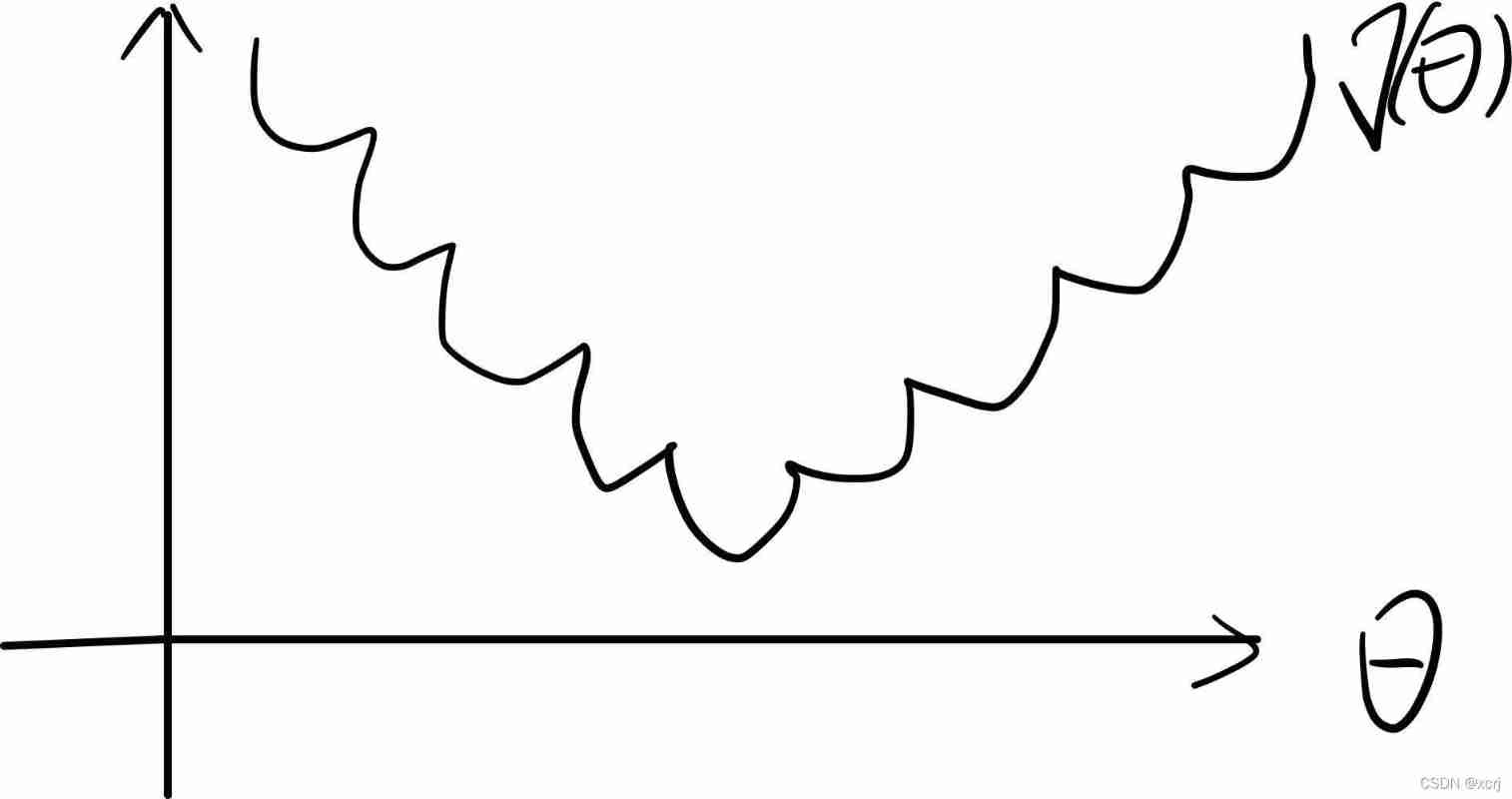
The original cost function :
- The original cost function cannot be used , Because there are too many local optima
- J ( θ ) = 1 m ∑ i = 1 m ( h θ ( x ( i ) ) − y ( i ) ) 2 J(\theta)=\frac{1}{m}\sum\limits_{i=1}^m(h_\theta(x^{(i)})-y^{(i)})^2 J(θ)=m1i=1∑m(hθ(x(i))−y(i))2, 0 ≤ h θ ( x ( i ) ≤ 1 0\leq h_\theta(x^{(i)} \leq1 0≤hθ(x(i)≤1 And y = 0 or 1 y=0 or 1 y=0 or 1, Lead to the existence of too many local optima , Not a typical convex function
New cost function : Converse thinking
c o s t ( h θ ( x ) , y ) = { − log ( h θ ( x ) ) y = 1 − log ( 1 − h θ ( x ) ) y = 0 cost(h_\theta(x),y)= \begin{cases} -\log(h_\theta(x))& y=1 \\ -\log(1-h_\theta(x))& y=0 \end{cases} cost(hθ(x),y)={ −log(hθ(x))−log(1−hθ(x))y=1y=0
Introduce
- l
y = 1 when { h θ ( x ) → 1 Such as fruit want h θ ( x ) → 0 be c o s t → + ∞ y=1 when \begin{cases} h_\theta(x)\rightarrow1 \\ If you want to h_\theta(x)\rightarrow0 be cost\rightarrow+\infty \end{cases} y=1 when { hθ(x)→1 Such as fruit want hθ(x)→0 be cost→+∞ - r
y = 0 when { h θ ( x ) → 0 Such as fruit want h θ ( x ) → 1 be c o s t → + ∞ y=0 when \begin{cases} h_\theta(x)\rightarrow0 \\ If you want to h_\theta(x)\rightarrow1 be cost\rightarrow+\infty \end{cases} y=0 when { hθ(x)→0 Such as fruit want hθ(x)→1 be cost→+∞
Unified cost function :
- c o s t ( h θ ( x ) , y ) = − y log ( h θ ( x ) ) − ( 1 − y ) log ( 1 − h θ ( x ) ) cost(h_\theta(x),y)=-y\log(h_\theta(x))-(1-y)\log(1-h_\theta(x)) cost(hθ(x),y)=−ylog(hθ(x))−(1−y)log(1−hθ(x))
- When y=1 when , Keep the front of the above formula 1 part
- When y=0 when , Keep the last of the above formula 1 part
cost function : Least square method
J ( θ ) = 1 m ∑ i = 1 m c o s t ( h θ ( x ) , y ) = 1 m ∑ i = 1 m [ − y log ( h θ ( x ) ) − ( 1 − y ) log ( 1 − h θ ( x ) ) ] \begin{aligned} J(\theta) &=\frac{1}{m}\sum\limits_{i=1}^mcost(h_\theta(x),y) \\ &=\frac{1}{m}\sum\limits_{i=1}^m[-y\log(h_\theta(x))-(1-y)\log(1-h_\theta(x))] \end{aligned} J(θ)=m1i=1∑mcost(hθ(x),y)=m1i=1∑m[−ylog(hθ(x))−(1−y)log(1−hθ(x))]
Batch gradient descent algorithm :
- Repeat until it converges {
θ 0 : = θ 0 − α ∂ J ( θ ) ∂ θ 0 \theta_0:=\theta_0-\alpha\frac{\partial{J(\theta)}}{\partial{\theta_0}} θ0:=θ0−α∂θ0∂J(θ)
θ j : = θ j − α ∂ J ( θ ) ∂ θ j \theta_j:=\theta_j-\alpha\frac{\partial{J(\theta)}}{\partial{\theta_j}} θj:=θj−α∂θj∂J(θ)
} - Repeat until it converges {
θ 0 : = θ 0 − α 1 m ∑ i = 1 m [ h θ ( x ) − y ] \theta_0:=\theta_0-\alpha\frac{1}{m}\sum\limits_{i=1}^m[h_\theta(x)-y] θ0:=θ0−αm1i=1∑m[hθ(x)−y]
θ j : = θ j − α 1 m ∑ i = 1 m [ h θ ( x ) − y ] x j \theta_j:=\theta_j-\alpha\frac{1}{m}\sum\limits_{i=1}^m[h_\theta(x)-y]x_j θj:=θj−αm1i=1∑m[hθ(x)−y]xj
} - Be careful : Batch gradient descent algorithm needs to update all at the same time θ j \theta_j θj
Data sets
Spam differentiation
- Address download spambase.data File can
- Dichotomous problem :spam or non-spam
- This experiment only takes the first 3 Columns as features , Last 1 Column as the target , Last 1 The column value is 1 when spam, Last 1 The column value is 0 when non-spam,
Code
from mpl_toolkits.mplot3d import Axes3D
import pandas as pd
import numpy as np
import matplotlib
import matplotlib.pyplot as plt

matplotlib.rcParams['font.family'] = 'STSong'
matplotlib.rcParams['font.size'] = 20


class DataSet(object):
    """ X_train  Training set samples  y_train  Training set sample value  X_test  Test set samples  y_test  Test set sample values  """

    def __init__(self, X_train, y_train, X_test, y_test):
        self.X_train = X_train
        self.y_train = y_train
        self.X_test = X_test
        self.y_test = y_test


class LogisticRegression(object):
    """  Logical regression  """

    def __init__(self, n_feature):
        self.theta0 = 0
        self.theta = np.zeros((n_feature, 1))

    def sigmoid(self, z):
        return 1 / (1 + np.exp(-z))

    def gradient_descent(self, X, y, alpha=0.001, num_iter=100):
        costs = []
        m, _ = X.shape
        for i in range(num_iter):
            #  Predictive value
            h = self.sigmoid(np.dot(X, self.theta) + self.theta0)
            #  cost function
            cost = (1 / m) * np.sum(-y * np.log(h) - (1 - y) * (np.log(1 - h)))
            costs.append(cost)
            #  gradient
            dJ_dtheta0 = (1 / m) * np.sum(h - y)
            dJ_dtheta = (1 / m) * np.dot((h - y).T, X).T
            #  Update all at the same time theta
            self.theta0 = self.theta0 - alpha * dJ_dtheta0
            self.theta = self.theta - alpha * dJ_dtheta

        return costs

    def show_train(self, costs, num_iter):
        """  Show the training process  """
        fig = plt.figure(figsize=(10, 6))
        plt.plot(np.arange(num_iter), costs)
        plt.title(" Cost changes ")
        plt.xlabel(" The number of iterations ")
        plt.ylabel(" cost ")
        plt.show()

    def hypothesis(self, X, theta0, theta):
        """  Prediction function  """
        h0 = self.sigmoid(self.theta0 + np.dot(X, self.theta))
        h = [1 if elem > 0.5 else 0 for elem in h0]
        return np.array(h)[:, np.newaxis]


def read_data():
    """  Reading data  """
    # names: Header
    # sep: Separator
    # skipinitialspace: Ignore the space after the delimiter
    # comment: Ignore \t Note after
    # na_values: Use ? Replace NA Value
    origin_data = pd.read_csv("./data/spambase.data", sep=",", skipinitialspace=True, comment="\t", na_values="?")
    data = origin_data.copy()
    # tail() Print last n Row data
    print(data.tail())
    return data


def clean_data(data):
    """  Data cleaning : Handling outliers  """
    # dataset Does it contain NA data
    # pandas 0.22.0+ Only then isna(), Upgrade order :pip install --upgrade pandas==0.22.0
    print('NA Row number :', data.isna().sum())
    #  Delete the exception line
    cleaned_data = data.dropna()
    return cleaned_data


def show_data(data):
    """  Show the data  """
    count_spam = 0
    count_non_spam = 0
    for c in data.iloc[:, -1]:
        if c == 1:
            count_spam += 1
        else:
            count_non_spam += 1

    print(" Number of spam :", count_spam)
    print(" Number of normal mail :", count_non_spam)


def split_data(data):
    """  Divide the data   Divided into train, test;train Used to train the prediction function ,test Used to test the generalization ability of the predicted function value  """
    copied_data = data.copy()
    # frac: The proportion of rows extracted ;random_state  Random seeds
    train_dataset = copied_data.sample(frac=0.8, random_state=1)
    #  Take the rest of the test set
    test_dataset = copied_data.drop(train_dataset.index)

    X_train = train_dataset.iloc[:, 0:3]
    y_train = train_dataset.iloc[:, -1]
    X_test = test_dataset.iloc[:, 0:3]
    y_test = test_dataset.iloc[:, -1]
    dataset = DataSet(X_train, y_train, X_test, y_test)

    return dataset


def evaluate_model(y_test, h):
    """  Evaluation model  """
    # MSE: Mean square error
    print("MSE: %f" % (np.sum((h - y_test) ** 2) / len(y_test)))
    # RMSE: Root mean square difference
    print("RMSE: %f" % (np.sqrt(np.sum((h - y_test) ** 2) / len(y_test))))

def show_result(X_test, y_test, h):
    # figure canvas
    fig = plt.figure(figsize=(16, 8), facecolor='w')
    # subplot Subgraphs
    plt.subplots_adjust(left=0.05, right=0.95, bottom=0.05, top=0.9)

    # 221:nrows=2, ncols=2, index=1
    ax = fig.add_subplot(121, projection='3d')
    ax.set_title("y_test")
    ax.set_xlabel('Feature 1')
    ax.set_ylabel('Feature 2')
    ax.set_zlabel('Feature 3')
    # x,y,z,c(color),marker( shape )
    ax.scatter(X_test[:, 0], X_test[:, 1], X_test[:, 2], c=y_test, marker='o')
    plt.grid(True)

    ax1 = fig.add_subplot(122, projection='3d')
    ax1.set_title("h")
    ax1.set_xlabel('Feature 1')
    ax1.set_ylabel('Feature 2')
    ax1.set_zlabel('Feature 3')
    # x,y,z,c(color),marker( shape )
    ax1.scatter(X_test[:, 0], X_test[:, 1], X_test[:, 2], c=h, marker='*')
    plt.grid(True)

    plt.show()

def main():
    #  Reading data
    data = read_data()
    #  Data cleaning
    cleaned_data = clean_data(data)
    #  Mean normalization , Before the data set used 3 There is little difference in the range of column data , Do not normalize the mean
    #  Display data
    show_data(cleaned_data)
    #  Split data
    dataset = split_data(cleaned_data)
    #  Build the model
    _, n = dataset.X_train.shape
    logistic_regression = LogisticRegression(n)
    num_iteration = 300
    costs = logistic_regression.gradient_descent(dataset.X_train, dataset.y_train.values[:, np.newaxis], alpha=0.5,
                                                 num_iter=num_iteration)
    #  Show the training process
    logistic_regression.show_train(costs, num_iteration)
    #  Evaluation model
    h = logistic_regression.hypothesis(dataset.X_test, logistic_regression.theta0, logistic_regression.theta)
    evaluate_model(dataset.y_test.values[:, np.newaxis], h)
    #  Display the results
    show_result(dataset.X_test.values,dataset.y_test.values, h.ravel())


if __name__ == '__main__':
    main()
边栏推荐
- From starfish OS' continued deflationary consumption of SFO, the value of SFO in the long run
- 第七章 行为级建模
- metasploit
- 给刚入门或者准备转行网络工程师的朋友一些建议
- C语言-模块化-Clion(静态库,动态库)使用
- QT -- create QT program
- List of top ten domestic industrial 3D visual guidance enterprises in 2022
- Gbase observation | how to protect the security of information system with frequent data leakage
- Keras' deep learning practice -- gender classification based on inception V3
- 日志特征选择汇总(基于天池比赛)
猜你喜欢

云原生应用开发之 gRPC 入门
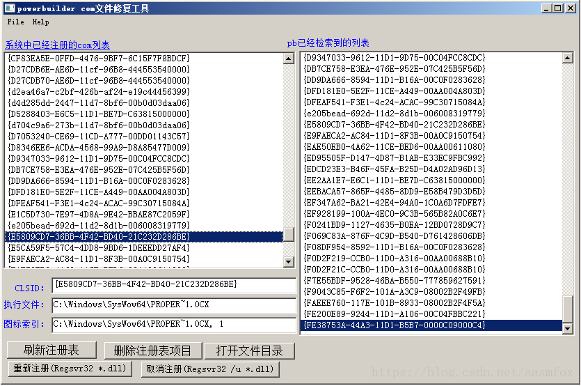
pb9.0 insert ole control 错误的修复工具
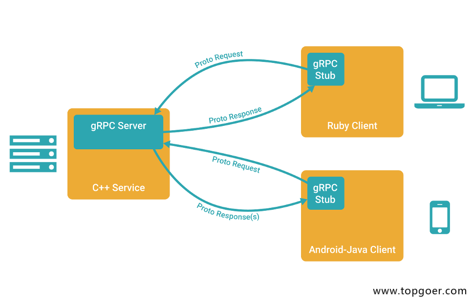
Introduction to grpc for cloud native application development

Partage d'expériences de contribution à distance

Reading notes of Clickhouse principle analysis and Application Practice (7)
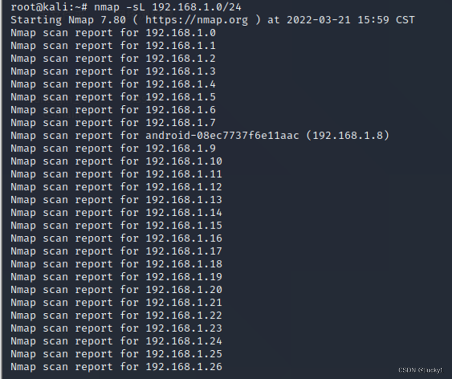
nmap工具介紹及常用命令
![[target tracking] |atom](/img/33/529b483a0a848e0e4263ba24462d5c.png)
[target tracking] |atom

Exit of processes and threads
metasploit

COMSOL --- construction of micro resistance beam model --- final temperature distribution and deformation --- addition of materials
随机推荐
Gbase observation | how to protect the security of information system with frequent data leakage
Kwai applet guaranteed payment PHP source code packaging
In depth analysis of ArrayList source code, from the most basic capacity expansion principle, to the magic iterator and fast fail mechanism, you have everything you want!!!
Uniapp one click Copy function effect demo (finishing)
nmap工具介紹及常用命令
Optimization of ecological | Lake Warehouse Integration: gbase 8A MPP + xeos
电路如图,R1=2kΩ,R2=2kΩ,R3=4kΩ,Rf=4kΩ。求输出与输入关系表达式。
Redisson分布式锁解锁异常
cv2读取视频-并保存图像或视频
软件测试笔试题你会吗?
用户之声 | 冬去春来,静待花开 ——浅谈GBase 8a学习感悟
Nacos microservice gateway component +swagger2 interface generation
The circuit is shown in the figure, r1=2k Ω, r2=2k Ω, r3=4k Ω, rf=4k Ω. Find the expression of the relationship between output and input.
The foreach map in JS cannot jump out of the loop problem and whether foreach will modify the original array
If time is a river
腾讯游戏客户端开发面试 (Unity + Cocos) 双重轰炸 社招6轮面试
Partage d'expériences de contribution à distance
PHP calculates personal income tax
MySQL查询为什么没走索引?这篇文章带你全面解析
第七章 行为级建模