当前位置:网站首页>Mobile robot path planning: artificial potential field method [easy to understand]
Mobile robot path planning: artificial potential field method [easy to understand]
2022-07-02 19:21:00 【Full stack programmer webmaster】
Hello everyone , I meet you again , I'm your friend, Quan Jun .
The artificial potential field method is a simple method Move robot Path planning algorithm , It regards the position of the target point as the lowest point of potential energy , Treat obstacles in the map as potential energy highs , Calculate the potential field diagram of the whole known map , And then, ideally , The robot is like a rolling ball , Automatically avoid all obstacles and roll to the target point .
- Reference resources : Source code potential_field_planning.py Courseware CMU RI 16-735 Robot path planning 4 speak : Artificial potential field method
In particular , The potential energy formula of the target point is :
It reads , In order to prevent the speed from being too fast when it is far away from the target point , It can be described in the form of piecewise function , It will be shown later . The potential energy of the obstacle is expressed as :
That is, it has high potential energy in a certain range around the obstacle , The influence of out of range visual obstacles is 0. Finally, add the potential energy of the target point and the obstacle , Get the whole potential energy map :
The following is the source code in the reference link , It's easier to understand :
""" Potential Field based path planner author: Atsushi Sakai (@Atsushi_twi) Ref: https://www.cs.cmu.edu/~motionplanning/lecture/Chap4-Potential-Field_howie.pdf """

from collections import deque
import numpy as np
import matplotlib.pyplot as plt

# Parameters
KP = 5.0  # attractive potential gain
ETA = 100.0  # repulsive potential gain
AREA_WIDTH = 30.0  # potential area width [m]
# the number of previous positions used to check oscillations
OSCILLATIONS_DETECTION_LENGTH = 3

show_animation = True


def calc_potential_field(gx, gy, ox, oy, reso, rr, sx, sy):
    """  Calculate the potential field diagram  gx,gy:  Target coordinates  ox,oy:  Obstacle coordinate list  reso:  Potential field diagram resolution  rr:  Robot radius  sx,sy:  Starting point coordinates  """
    #  Determine the coordinate range of the potential field diagram :
    minx = min(min(ox), sx, gx) - AREA_WIDTH / 2.0
    miny = min(min(oy), sy, gy) - AREA_WIDTH / 2.0
    maxx = max(max(ox), sx, gx) + AREA_WIDTH / 2.0
    maxy = max(max(oy), sy, gy) + AREA_WIDTH / 2.0
    #  Determine the number of cells according to the range and resolution :
    xw = int(round((maxx - minx) / reso))
    yw = int(round((maxy - miny) / reso))

    # calc each potential
    pmap = [[0.0 for i in range(yw)] for i in range(xw)]

    for ix in range(xw):
        x = ix * reso + minx   #  According to index and resolution x coordinate

        for iy in range(yw):
            y = iy * reso + miny  #  According to index and resolution x coordinate
            ug = calc_attractive_potential(x, y, gx, gy)  #  Calculate gravity
            uo = calc_repulsive_potential(x, y, ox, oy, rr)  #  Calculated repulsion
            uf = ug + uo
            pmap[ix][iy] = uf

    return pmap, minx, miny


def calc_attractive_potential(x, y, gx, gy):
    """  Calculate the gravitational potential energy :1/2*KP*d """
    return 0.5 * KP * np.hypot(x - gx, y - gy)


def calc_repulsive_potential(x, y, ox, oy, rr):
    """  Calculate the repulsive potential energy :  If the distance from the nearest obstacle dq In the robot expansion radius rr within :1/2*ETA*(1/dq-1/rr)**2  otherwise :0.0 """
    # search nearest obstacle
    minid = -1
    dmin = float("inf")
    for i, _ in enumerate(ox):
        d = np.hypot(x - ox[i], y - oy[i])
        if dmin >= d:
            dmin = d
            minid = i

    # calc repulsive potential
    dq = np.hypot(x - ox[minid], y - oy[minid])

    if dq <= rr:
        if dq <= 0.1:
            dq = 0.1

        return 0.5 * ETA * (1.0 / dq - 1.0 / rr) ** 2
    else:
        return 0.0


def get_motion_model():
    # dx, dy
    #  Jiugonggezhong  8 Possible directions of motion
    motion = [[1, 0],
              [0, 1],
              [-1, 0],
              [0, -1],
              [-1, -1],
              [-1, 1],
              [1, -1],
              [1, 1]]

    return motion


def oscillations_detection(previous_ids, ix, iy):
    """  Oscillation detection : avoid “ Repeat the cross jump ” """
    previous_ids.append((ix, iy))

    if (len(previous_ids) > OSCILLATIONS_DETECTION_LENGTH):
        previous_ids.popleft()

    # check if contains any duplicates by copying into a set
    previous_ids_set = set()
    for index in previous_ids:
        if index in previous_ids_set:
            return True
        else:
            previous_ids_set.add(index)
    return False


def potential_field_planning(sx, sy, gx, gy, ox, oy, reso, rr):

    # calc potential field
    pmap, minx, miny = calc_potential_field(gx, gy, ox, oy, reso, rr, sx, sy)

    # search path
    d = np.hypot(sx - gx, sy - gy)
    ix = round((sx - minx) / reso)
    iy = round((sy - miny) / reso)
    gix = round((gx - minx) / reso)
    giy = round((gy - miny) / reso)

    if show_animation:
        draw_heatmap(pmap)
        # for stopping simulation with the esc key.
        plt.gcf().canvas.mpl_connect('key_release_event',
                lambda event: [exit(0) if event.key == 'escape' else None])
        plt.plot(ix, iy, "*k")
        plt.plot(gix, giy, "*m")

    rx, ry = [sx], [sy]
    motion = get_motion_model()
    previous_ids = deque()

    while d >= reso:
        minp = float("inf")
        minix, miniy = -1, -1
        #  seek 8 The direction in which the potential field is the smallest among the three directions of motion
        for i, _ in enumerate(motion):
            inx = int(ix + motion[i][0])
            iny = int(iy + motion[i][1])
            if inx >= len(pmap) or iny >= len(pmap[0]) or inx < 0 or iny < 0:
                p = float("inf")  # outside area
                print("outside potential!")
            else:
                p = pmap[inx][iny]
            if minp > p:
                minp = p
                minix = inx
                miniy = iny
        ix = minix
        iy = miniy
        xp = ix * reso + minx
        yp = iy * reso + miny
        d = np.hypot(gx - xp, gy - yp)
        rx.append(xp)
        ry.append(yp)
        #  Oscillation detection , To avoid falling into a local minimum :
        if (oscillations_detection(previous_ids, ix, iy)):
            print("Oscillation detected at ({},{})!".format(ix, iy))
            break

        if show_animation:
            plt.plot(ix, iy, ".r")
            plt.pause(0.01)

    print("Goal!!")

    return rx, ry


def draw_heatmap(data):
    data = np.array(data).T
    plt.pcolor(data, vmax=100.0, cmap=plt.cm.Blues)


def main():
    print("potential_field_planning start")

    sx = 0.0  # start x position [m]
    sy = 10.0  # start y positon [m]
    gx = 30.0  # goal x position [m]
    gy = 30.0  # goal y position [m]
    grid_size = 0.5  # potential grid size [m]
    robot_radius = 5.0  # robot radius [m]
    #  The following obstacle coordinates are my modified , It is used to show the situation that the artificial potential field method is trapped in local optimization :
    ox = [15.0, 5.0, 20.0, 25.0, 12.0, 15.0, 19.0, 28.0, 27.0, 23.0, 30.0, 32.0]  # obstacle x position list [m]
    oy = [25.0, 15.0, 26.0, 25.0, 12.0, 20.0, 29.0, 28.0, 26.0, 25.0, 28.0, 27.0]  # obstacle y position list [m]

    if show_animation:
        plt.grid(True)
        plt.axis("equal")

    # path generation
    _, _ = potential_field_planning(
        sx, sy, gx, gy, ox, oy, grid_size, robot_radius)

    if show_animation:
        plt.show()


if __name__ == '__main__':
    print(__file__ + " start!!")
    main()
print(__file__ + " Done!!")One of the main disadvantages of the artificial potential field method is that it may fall into the local optimal solution , The following figure is the result of running the source code :
Here is after I added some obstacles , The artificial potential field method is trapped in the case of local optimal solution : Although the target point has not been reached , But the potential field determines that the path cannot go any further .
It should be noted that , When calculating the potential field of the target point in the source code , It uses a x,y A term of the distance between the position and the target point , The quadratic term is not used as shown in the courseware , It is also to make the potential field change less quickly . The following is according to the courseware , The result of using the quadratic term of distance , We can see , For normal operation ,KP It needs to be adjusted very low :
KP = 0.1
def calc_attractive_potential(x, y, gx, gy):
    """  Calculate the gravitational potential energy :1/2*KP*d^2 """
return 0.5 * KP * np.hypot(x - gx, y - gy)**2The normal operation :
Trapped in local best :
You can see from the potential field diagram , Gravity changes much faster than the previous example .
Last , We modify the program into the segmentation function shown in the screenshot of the courseware above :
KP = 0.25
dgoal = 10
def calc_attractive_potential(x, y, gx, gy):
    """  Calculate gravity : Such as courseware screenshot  """
    dg = np.hypot(x - gx, y - gy)
    if dg<=dgoal:
        U = 0.5 * KP * np.hypot(x - gx, y - gy)**2
    else:
        U = dgoal*KP*np.hypot(x - gx, y - gy) - 0.5*KP*dgoal
return UThe normal operation :
Trapped in local optima :
You can see the effect of gravitational potential field segmentation .
Publisher : Full stack programmer stack length , Reprint please indicate the source :https://javaforall.cn/148611.html Link to the original text :https://javaforall.cn
边栏推荐
- C file input operation
- yolov3 训练自己的数据集之生成train.txt
- R language ggplot2 visual Facet: gganimate package is based on Transition_ Time function to create dynamic scatter animation (GIF)
- Machine learning notes - time series prediction research: monthly sales of French champagne
- [paper reading] Ca net: leveraging contextual features for lung cancer prediction
- Qpropertyanimation use and toast case list in QT
- 新手必看,點擊兩個按鈕切換至不同的內容
- Learning summary of MySQL advanced 6: concept and understanding of index, detailed explanation of b+ tree generation process, comparison between MyISAM and InnoDB
- Crypto usage in nodejs
- 仿京东放大镜效果(pink老师版)
猜你喜欢
使用CLion编译OGLPG-9th-Edition源码
![[daily question] first day](/img/8c/f25cddb6ca86d44538c976fae13c6e.png)
[daily question] first day
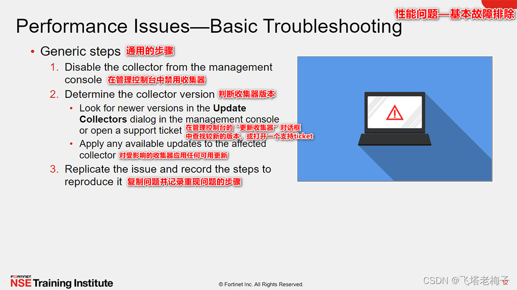
Tutoriel (5.0) 10. Dépannage * fortiedr * fortinet Network Security expert NSE 5
Tutorial (5.0) 10 Troubleshooting * fortiedr * Fortinet network security expert NSE 5
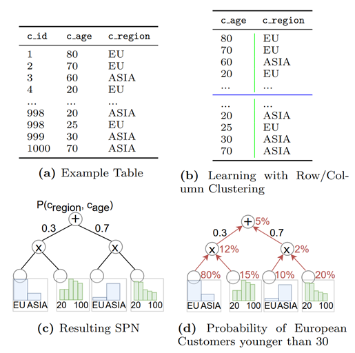
Introduction to the paper | application of machine learning in database cardinality estimation
![[daily question] the next day](/img/8a/18329bd9b4a3a4445c8fbbc1ce562b.png)
[daily question] the next day

Tutorial (5.0) 09 Restful API * fortiedr * Fortinet network security expert NSE 5
![[0701] [论文阅读] Alleviating Data Imbalance Issue with Perturbed Input During Inference](/img/c7/9b7dc4b4bda4ecfe07aec1367fe059.png)
[0701] [论文阅读] Alleviating Data Imbalance Issue with Perturbed Input During Inference

Why should we build an enterprise fixed asset management system and how can enterprises strengthen fixed asset management
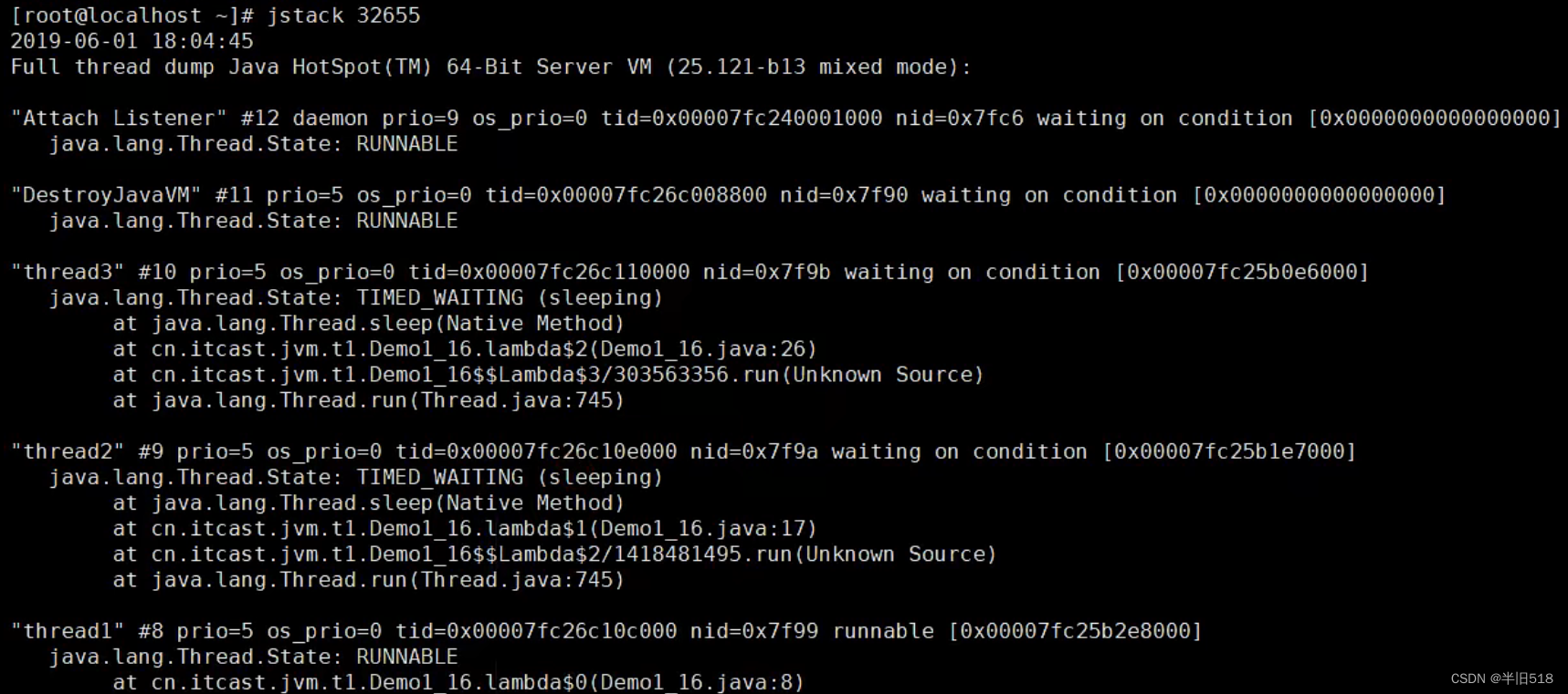
【JVM调优实战100例】02——虚拟机栈与本地方法栈调优五例
随机推荐
Date tool class (updated from time to time)
ICDE 2023|TKDE Poster Session(CFP)
Emmet基础语法
Codeworks 5 questions per day (1700 average) - day 4
SIFT特征点提取「建议收藏」
2022 software engineering final exam recall Edition
Data dimensionality reduction principal component analysis
二进制操作
2022 compilation principle final examination recall Edition
reduce--遍历元素计算 具体的计算公式需要传入 结合BigDecimal
Markdown基础语法
QT中的QPropertyAnimation使用和toast案列
Reduce -- traverse element calculation. The specific calculation formula needs to be passed in and combined with BigDecimal
Markdown basic grammar
ICDE 2023|TKDE Poster Session(CFP)
Page title component
Mysql高级篇学习总结8:InnoDB数据存储结构页的概述、页的内部结构、行格式
A4988驱动步进电机「建议收藏」
Kubernetes three open interfaces first sight
Progress-进度条