Machine learning notes - time series as features

One 、 Serial dependency

         Attributes of time series that are most easily modeled as time-dependent attributes , in other words , We can get features directly from the time index . however , Some time series attributes can only be modeled as series related attributes , That is, the past value of the target sequence is used as the feature . as time goes on , The structure of these time series may not be obvious ; However , Draw based on past values , The structure becomes clear - As shown in the figure below .

These two families have sequence dependencies , But it is not time dependent . The point on the right has coordinates （ Time t-1 Value , Time t Value ）.

          With trends and seasonality , We trained the model to fit the curve to the graph on the left of the above figure —— These models are learning about time dependency .

1、 loop

         A particularly common way to represent serial dependencies is through loops . Periods are growth and decay patterns in time series , It is related to how the value in a sequence depends on the value of the previous time , But it doesn't necessarily depend on the time step itself . Cyclic behavior is a characteristic of a system that can affect itself or its response over time . economic 、 Epidemic 、 Animal populations 、 Volcanic eruptions and similar natural phenomena often exhibit cyclic behavior .

         The difference between cyclical behavior and seasonality is , Cycles do not necessarily depend on time as seasons do . What happens in a cycle has nothing to do with a specific date , And it's more about recent events . With time （ At least relative ） Independence means that circular behavior may be more irregular than seasonality . 

Two 、 Lag sequence and lag graph

         To investigate possible sequence dependencies in time series （ Such as period ）, We need to create a sequence “ lagging ” copy . A lag time series means moving its value forward by one or more time steps , Or equivalent , Moves the time in its index backward by one or more steps . In any case , The result is that the observations in the lag series seem to occur at a later time .

         This shows the monthly unemployment rate (y) And its first and second lag sequences （ Respectively y_lag_1 and y_lag_2）. Notice how the value of the lag sequence moves forward in time .

import pandas as pd

# Federal Reserve dataset: https://www.kaggle.com/federalreserve/interest-rates
reserve = pd.read_csv(
    "../input/ts-course-data/reserve.csv",
    parse_dates={'Date': ['Year', 'Month', 'Day']},
    index_col='Date',
)

y = reserve.loc[:, 'Unemployment Rate'].dropna().to_period('M')
df = pd.DataFrame({
    'y': y,
    'y_lag_1': y.shift(1),
    'y_lag_2': y.shift(2),    
})

df.head()

Date	y	y_lag_1	y_lag_2
1954-07	5.8	NaN	NaN
1954-08	6.0	5.8	NaN
1954-09	6.1	6.0	5.8
1954-10	5.7	6.1	6.0
1954-11	5.3	5.7	6.1

         Through lag time series , We can make its past value appear at the same time as the value we are trying to predict （ let me put it another way , In the same line ）. This makes the lag sequence available as a feature for modeling sequence dependencies . To predict the unemployment rate series , We can use y_lag_1 and y_lag_2 As a feature to predict the target y. This will forecast the future unemployment rate as a function of the unemployment rate in the previous two months .

1、 Lag graph

         The lag graph of the time series shows the plotted values relative to the lag . By looking at the lag graph , The sequence dependence in time series usually becomes obvious . We can see from this lagging chart of the US unemployment rate , There is a strong and obvious linear relationship between the current unemployment rate and the past unemployment rate .

Unemployment lag graph showing autocorrelation .

          The most common measure of sequence dependence is called autocorrelation , It is only the correlation between time series and one of their lags . The unemployment rate is lagging behind 1 The autocorrelation of time is 0.99, It's lagging behind 2 When is 0.98, And so on .

2、 Choice lag

         When selecting hysteresis as a feature , It is often useless to include each lag in autocorrelation . for example , In the midst of unemployment , lagging 2 The autocorrelation of may come entirely from hysteresis 1 Of “ attenuation ” Information —— It is only the related information inherited from the previous step . If lag 2 Does not contain any new content , So if we already have a lag 1, There is no reason to include it .

         Partial autocorrelation tells you the correlation of the lag to all previous lags —— so to speak , Lagging contribution “ new ” Correlation quantity . Plotting partial autocorrelation can help you choose which hysteresis feature to use . In the following illustration , lagging 1 To lag 6 Fall in the “ No correlation ” Section （ Blue ） outside , So we can choose to lag 1 To lag 6 As a characteristic of the unemployment rate . （ lagging 11 It could be a false alarm .）

The partial autocorrelation of the unemployment rate through lag 12 Not related to 95% confidence interval .

          A graph like the one above is called a correlation graph . The correlation diagram is applicable to the hysteresis characteristics , It is essentially like a periodic graph applied to Fourier features .

         Last , We need to note that autocorrelation and partial autocorrelation are measures of linear correlation . Because the time series in the real world usually have great nonlinear correlation , Therefore, when selecting hysteresis characteristics , It's best to look at the lag chart （ Or use some more general correlation measures , Such as mutual information ）. The sunspot series have nonlinear related hysteresis , We may ignore autocorrelation .

Hysteresis diagram of sunspot series .

          A nonlinear relationship like this can be transformed into a linear relationship , You can also learn through appropriate algorithms .

3、 ... and 、 Example - Influenza trends

        Flu Trends Data set containing 2009 - 2016 A doctor's record of seeing a doctor for flu for several weeks over the years . Our goal is to predict the number of influenza cases in the coming weeks .

         We will take two approaches . First , We will use the lag feature to predict the number of doctor visits . Our second method is to use the lag of another set of time series to predict the number of doctor visits ： Google Trends captures flu related search terms .

from pathlib import Path
from warnings import simplefilter

import matplotlib.pyplot as plt
import numpy as np
import pandas as pd
import seaborn as sns
from scipy.signal import periodogram
from sklearn.linear_model import LinearRegression
from sklearn.model_selection import train_test_split
from statsmodels.graphics.tsaplots import plot_pacf

simplefilter("ignore")

# Set Matplotlib defaults
plt.style.use("seaborn-whitegrid")
plt.rc("figure", autolayout=True, figsize=(11, 4))
plt.rc(
    "axes",
    labelweight="bold",
    labelsize="large",
    titleweight="bold",
    titlesize=16,
    titlepad=10,
)
plot_params = dict(
    color="0.75",
    style=".-",
    markeredgecolor="0.25",
    markerfacecolor="0.25",
)
%config InlineBackend.figure_format = 'retina'


def lagplot(x, y=None, lag=1, standardize=False, ax=None, **kwargs):
    from matplotlib.offsetbox import AnchoredText
    x_ = x.shift(lag)
    if standardize:
        x_ = (x_ - x_.mean()) / x_.std()
    if y is not None:
        y_ = (y - y.mean()) / y.std() if standardize else y
    else:
        y_ = x
    corr = y_.corr(x_)
    if ax is None:
        fig, ax = plt.subplots()
    scatter_kws = dict(
        alpha=0.75,
        s=3,
    )
    line_kws = dict(color='C3', )
    ax = sns.regplot(x=x_,
                     y=y_,
                     scatter_kws=scatter_kws,
                     line_kws=line_kws,
                     lowess=True,
                     ax=ax,
                     **kwargs)
    at = AnchoredText(
        f"{corr:.2f}",
        prop=dict(size="large"),
        frameon=True,
        loc="upper left",
    )
    at.patch.set_boxstyle("square, pad=0.0")
    ax.add_artist(at)
    ax.set(title=f"Lag {lag}", xlabel=x_.name, ylabel=y_.name)
    return ax


def plot_lags(x, y=None, lags=6, nrows=1, lagplot_kwargs={}, **kwargs):
    import math
    kwargs.setdefault('nrows', nrows)
    kwargs.setdefault('ncols', math.ceil(lags / nrows))
    kwargs.setdefault('figsize', (kwargs['ncols'] * 2, nrows * 2 + 0.5))
    fig, axs = plt.subplots(sharex=True, sharey=True, squeeze=False, **kwargs)
    for ax, k in zip(fig.get_axes(), range(kwargs['nrows'] * kwargs['ncols'])):
        if k + 1 <= lags:
            ax = lagplot(x, y, lag=k + 1, ax=ax, **lagplot_kwargs)
            ax.set_title(f"Lag {k + 1}", fontdict=dict(fontsize=14))
            ax.set(xlabel="", ylabel="")
        else:
            ax.axis('off')
    plt.setp(axs[-1, :], xlabel=x.name)
    plt.setp(axs[:, 0], ylabel=y.name if y is not None else x.name)
    fig.tight_layout(w_pad=0.1, h_pad=0.1)
    return fig


data_dir = Path("../input/ts-course-data")
flu_trends = pd.read_csv(data_dir / "flu-trends.csv")
flu_trends.set_index(
    pd.PeriodIndex(flu_trends.Week, freq="W"),
    inplace=True,
)
flu_trends.drop("Week", axis=1, inplace=True)

ax = flu_trends.FluVisits.plot(title='Flu Trends', **plot_params)
_ = ax.set(ylabel="Office Visits")

          Our influenza trend data show irregular cycles rather than regular seasonality ： The peak often occurs around the new year , But sometimes earlier or later , Sometimes larger or smaller . Modeling these cycles using lag features will enable our forecasters to respond dynamically to changing conditions , Instead of being limited by the exact date and time as seasonal characteristics .

         Let's first look at the lag and autocorrelation graph ：

_ = plot_lags(flu_trends.FluVisits, lags=12, nrows=2)
_ = plot_pacf(flu_trends.FluVisits, lags=12)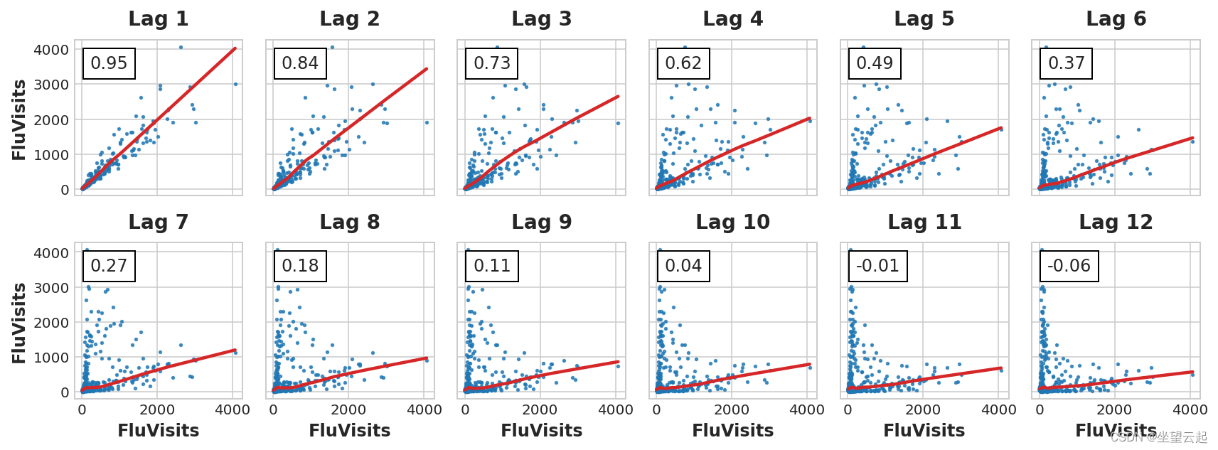

         The hysteresis diagram shows FluVisits The relationship with its lag is mainly linear , Partial autocorrelation indicates that hysteresis can be used 1、2、3 and 4 Capture dependencies . We can use shift Method lag Pandas Time series in . For this question , We will use 0.0 Fill in missing values created by lag .

def make_lags(ts, lags):
    return pd.concat(
        {
            f'y_lag_{i}': ts.shift(i)
            for i in range(1, lags + 1)
        },
        axis=1)


X = make_lags(flu_trends.FluVisits, lags=4)
X = X.fillna(0.0)

         We can create predictions for any number of steps beyond the training data . However , When hysteresis is used , We are limited to the time steps available to predict the lag value . Use lag on Monday 1 function , We can't predict Wednesday , Because of the lag required 1 The value is Tuesday , But it hasn't happened yet .

         For the current example , We will only use values from the test set .

# Create target series and data splits
y = flu_trends.FluVisits.copy()
X_train, X_test, y_train, y_test = train_test_split(X, y, test_size=60, shuffle=False)

# Fit and predict
model = LinearRegression()  # `fit_intercept=True` since we didn't use DeterministicProcess
model.fit(X_train, y_train)
y_pred = pd.Series(model.predict(X_train), index=y_train.index)
y_fore = pd.Series(model.predict(X_test), index=y_test.index)

ax = y_train.plot(**plot_params)
ax = y_test.plot(**plot_params)
ax = y_pred.plot(ax=ax)
_ = y_fore.plot(ax=ax, color='C3')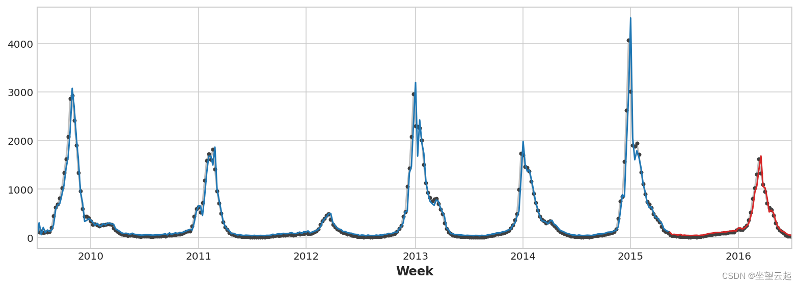

          Just look at the forecast , We can see how our model needs a time step to respond to sudden changes in the target sequence . This is a common limitation of models that only use the lag of the target series as a feature .

ax = y_test.plot(**plot_params)
_ = y_fore.plot(ax=ax, color='C3')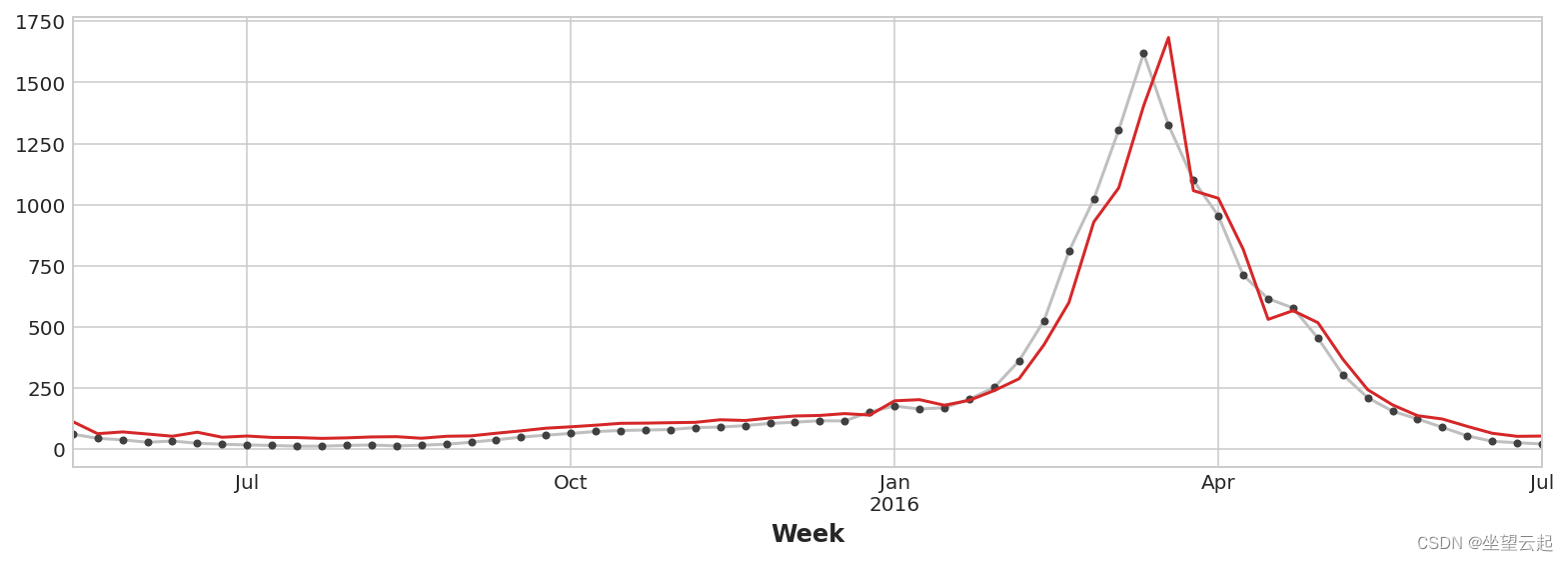

         To improve forecasting , We can try to find leading indicators , That is, it can provide information for the change of influenza cases “ early warning ” Time series of . For our second method , We will add to our training data the popularity of some flu related search terms measured by Google Trends .

         Will search for the phrase “FluCough” And target “FluVisits” Draw a chart to show , Such search terms may be useful as leading indicators ： Flu related searches tend to become more popular a few weeks before the visit .

ax = flu_trends.plot(
    y=["FluCough", "FluVisits"],
    secondary_y="FluCough",
)

          The dataset contains 129 Such a term , We only use a few of them .

search_terms = ["FluContagious", "FluCough", "FluFever", "InfluenzaA", "TreatFlu", "IHaveTheFlu", "OverTheCounterFlu", "HowLongFlu"]

# Create three lags for each search term
X0 = make_lags(flu_trends[search_terms], lags=3)

# Create four lags for the target, as before
X1 = make_lags(flu_trends['FluVisits'], lags=4)

# Combine to create the training data
X = pd.concat([X0, X1], axis=1).fillna(0.0)

         Our prediction is a bit rough , But our model seems to be better able to predict the sudden increase in influenza visits , This shows that several time series of search popularity are indeed effective as leading indicators .

X_train, X_test, y_train, y_test = train_test_split(X, y, test_size=60, shuffle=False)

model = LinearRegression()
model.fit(X_train, y_train)
y_pred = pd.Series(model.predict(X_train), index=y_train.index)
y_fore = pd.Series(model.predict(X_test), index=y_test.index)

ax = y_test.plot(**plot_params)
_ = y_fore.plot(ax=ax, color='C3')

         The time series in this paper can be called “ Pure cycle ”： They have no obvious trend or seasonality . Time series have trends at the same time 、 Seasonality and periodicity , Such sequences can be modeled using linear regression by adding appropriate features to each component . You can even mix models that have been trained to learn components separately .