当前位置:网站首页>Gradient epic memory for continuous learning
Gradient epic memory for continuous learning
2022-06-12 07:17:00 【Programmer long】
One . Introduce
At the beginning of supervised learning, we need to collect a training set D t r = { ( x i , y i ) } i = 1 n D_{tr}=\{(x_i,y_i)\}^n_{i=1} Dtr={ (xi,yi)}i=1n. Most supervised learning assumes that every example is from a fixed probability distribution P Independent identically distributed sampling in . The goal of supervised learning is to construct a model f f f To predict the target vector y adopt x. In order to realize this assumption , Supervised learning usually adopts the principle of empirical risk minimization (ERM), f f f In this case 1 ∣ D t r ∣ ∑ ( x i , y i ) ∈ D t r l ( f ( x i ) , y i ) \frac{1}{|D_{tr}|}\sum_{(x_i,y_i) \in D_{tr}}l(f(x_i),y_i) ∣Dtr∣1∑(xi,yi)∈Dtrl(f(xi),yi). actually ,ERM The training set needs to be traversed many times .
ERM It is a simplification of what we think of as human learning . However, in reality, people's observation is orderly , And the same example intelligently remembers a small amount of data . therefore ,iid Assumptions and any use ERM The hopes of principle were dashed . in other words ERM It will lead to disastrous forgetting .
This article reduces the ERM And human learning . It is worth noting that , The author is learning one by one , Arrive in order .
( x 1 , t 1 , y 1 ) , . . . , ( x i , t i , y i ) , . . . , ( x n , t n . y n ) (1) (x_1,t_1,y_1),...,(x_i,t_i,y_i),...,(x_n,t_n.y_n) \tag{1} (x1,t1,y1),...,(xi,ti,yi),...,(xn,tn.yn)(1)
Based on this situation , Facing ERM Unknown challenges :
- Non-iid Input data for : Data continuity for any fixed probability distribution P ( X , T , Y ) P(X,T,Y) P(X,T,Y) It's all uncertain , Because once the task switches , You can observe a series of examples from the new task .
- Catastrophic oblivion : Learning a new task may impair the learner's performance in a task that has been previously solved
- The migration study : When successive tasks are interrelated , There are opportunities for transfer learning . This translates into faster learning of new tasks , To improve the performance of old tasks .
Two . The framework of continuous learning
according to (1) The data described in , We assume that the continuous task distribution is local iid, That is to say, every ( x i , t i , y i ) (x_i,t_i,y_i) (xi,ti,yi) All satisfied with ( x i , y i ) ~ i i d P t i ( X , Y ) (x_i,y_i)~_{iid}P_{t_i}(X,Y) (xi,yi)~iidPti(X,Y). Our goal is to learn a model f f f, Be able to predict at any time , Such tests can belong to tasks we have observed in the past , Current tasks or tasks we will experience in the future .
Task descriptor : In the process of sequential tasks , Task descriptors are critical . Rich descriptors provide opportunities for zero learning , Therefore, new task descriptors can be used to infer between tasks . Besides , The task descriptor eliminates the ambiguity of similar learning tasks . In this article, we focus more on mitigating catastrophic forgetting , Learn from a continuous set of data and leave zero learning opportunities for future research .
Training protocol and evaluation indicators
In this paper , The task sequence considered is set as follows :a. The number of tasks is very large ,b. There are few training examples for each task ,c. Learners only observe examples of each task once ,d. Indicators to measure migration and forgetting are reported .
therefore , In training , We only give one example at a time ( Or a mini-batch) To learners . At the same time, learners will not experience the same example twice , And the hot dance is performed in sequence . There is no need to impose any order on the task , Because the tasks of the future may coincide with those of the past .
In addition to monitoring learners' cross task performance , It is also important to assess learners' ability to transfer knowledge , More specifically , Need to measure :
- Backward migration (BWT). This factor is mainly for learning tasks t And then look at t Performance of previous tasks . One side , Learning some tasks will improve the performance of the previous task , Positive post migration exists . Some will lead to negative migration . A large number of negative migrations will lead to catastrophic forgetting .
- Forward migration (FWT). This factor is the learning task t Then, let's look at the performance of the model in future task learning .
For the evaluation of the above principles , Consider right T Access to test sets for each of the tasks . When a model completes its task t i t_i ti after , We need to evaluate his test performance ability for all (T) The task of . After doing that , We can construct a matrix R ∈ R T ∗ T R\in \mathbb{R}^{T*T} R∈RT∗T, among R i , j R_{i,j} Ri,j Expressed as the accuracy of the test for the task t j t_j tj After observing the last one from t i t_i ti Example . Give Way b ˉ \bar{b} bˉ Test precision vector at random initialization for each task , We can define three matrices :
A C C = 1 T ∑ i = 1 T R T , i (2) ACC = \frac{1}{T}\sum_{i=1}^TR_{T,i} \tag{2} ACC=T1i=1∑TRT,i(2)
B W T = 1 T − 1 ∑ i = 1 T − 1 R T , i − R i , i (3) BWT =\frac{1}{T-1}\sum_{i=1}^{T-1}R_{T,i}-R_{i,i} \tag{3} BWT=T−11i=1∑T−1RT,i−Ri,i(3)
B W T = 1 T − 1 ∑ i = 2 T − 1 R i − 1 , i − b ˉ i (4) BWT =\frac{1}{T-1}\sum_{i=2}^{T-1}R_{i-1,i}-\bar{b}_i \tag{4} BWT=T−11i=2∑T−1Ri−1,i−bˉi(4)
3、 ... and . Episodic memory gradient (GEM)
GEM The main feature of the present study is an episodic memory M t \mathcal{M}_t Mt, Stored from task t A subset of the examples observed in . Next , It mainly focuses on minimizing negative transfer through the effective use of episodic memory ( Catastrophic oblivion ).
Actual summary , Learners share M Memory locations . If the number of tasks T It is known. , We can conclude that each task has m = M/T Of memory space . contrary , If the number of tasks is unknown , We need to keep reducing m For the new task . For the sake of simplicity , Let's assume that the memory is populated by the last example of each task , under these circumstances , Can be defined from k Scenario memory loss for tasks is :
l ( f θ , M k ) = 1 ∣ M k ∣ ∑ ( x i , k , y i ) ∈ M k l ( f θ ( x i , k ) , y i ) (5) l(f_\theta,\mathcal{M}_k)=\frac{1}{|\mathcal{M}_k|}\sum_{(x_i,k,y_i)\in \mathcal{M}_k}l(f_\theta(x_i,k),y_i) \tag{5} l(fθ,Mk)=∣Mk∣1(xi,k,yi)∈Mk∑l(fθ(xi,k),yi)(5)
obviously , Minimize current losses plus (5) It will lead to M \mathcal{M} M There is over fitting in . The author will use the loss (5) As a constraint of inequality , Avoid its increase but allow it to decrease . That is, the following description :
min θ l ( f θ ( x , t ) , y ) Its in l ( f θ , M k ) < = l ( f θ t − 1 , M k ) f o r a l l k < t , (6) \begin{aligned} \min_{\theta} \ \ \ &l(f_\theta(x,t),y) \\ among \ \ &l(f_\theta,\mathcal{M}_k)<=l(f_\theta^{t-1},\mathcal{M}_k) \ for\ all\ k<t,\tag{6} \end{aligned} θmin Its in l(fθ(x,t),y)l(fθ,Mk)<=l(fθt−1,Mk) for all k<t,(6)
Next , The author describes two important features to deal with the problem (6). The first is the , There is no need to store old models f θ t − 1 f_\theta^{t-1} fθt−1, As long as we guarantee that after each update , The loss of previous missions will not increase . second , Suppose the function is locally linear , Memory is a task that represents the past of an example , We can diagnose tasks with increased losses before , Calculate the angle between their loss vectors . therefore (6) It can be expressed as :
< g , g k > : = < ∂ l ( f θ ( x , t ) , y ) ∂ θ , ∂ l ( f θ , M k ) ∂ θ > > = 0 , f o r a l l k < t (7) <g,g_k>:=<\frac{\partial l(f_\theta(x,t),y)}{\partial\theta},\frac{\partial l(f_\theta,\mathcal{M}_k)}{\partial\theta}>\ >=0,for\ all\ k<t \tag{7} <g,gk>:=<∂θ∂l(fθ(x,t),y),∂θ∂l(fθ,Mk)> >=0,for all k<t(7)
If all are satisfied (7), Then parameter update g It is impossible to increase the loss of previous missions . in addition , If one or more are violated , Then at least one previous task will lose more after the parameter is updated . So you can take the gradient of violation g Project to the nearest gradient g ~ \tilde{g} g~( In square l2 standard ). therefore , Come here , The focus becomes :
min g ~ 1 2 ∣ ∣ g − g ~ ∣ ∣ 2 2 full foot < g ~ , g k > > = 0 f o r a l l k < t (8) \min_{\tilde{g}} \frac{1}{2}\ \ ||g-\tilde{g}||^2_2 \\ Satisfy <\tilde{g},g_k>\ \ >=0\ for\ all\ k<t \tag{8} g~min21 ∣∣g−g~∣∣22 full foot <g~,gk> >=0 for all k<t(8)
At this point, we can find that we only need to change our g ~ \tilde{g} g~ Make it form an acute angle with the vector of each previous task , And how to change this , The author turns the above question into 2 The problem of sub planning , However, the amount of calculation after conversion is too large , So the author changes to 2 The dual problem of sub programming is solved .
min z 1 2 v T G G T − g T z + g T G T v s u b j e c t t o v > = 0 (9) \min_z\ \frac{1}{2}v^TGG^T-g^Tz+g^TG^Tv \\ subject\ to \ \ v >=0 \tag{9} zmin 21vTGGT−gTz+gTGTvsubject to v>=0(9)
To calculate the v after , We can get our new g ~ = G T v + g \tilde{g} = G^Tv+g g~=GTv+g
The specific algorithm process is as follows :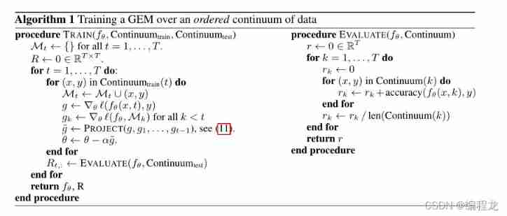
( In the picture 11 Corresponding to our formula 9)
Four . Code parsing
The author's code address is here
After reading it, you must be confused about the secondary planning , In fact, if you don't specialize in algorithms , You don't have to care so much , Because we just need to call the library .
Before starting the code again , Let's first think about this paper and the general DNN What's the difference? . The first is the , We need to store previous tasks ( That is to open up a space to store some of the previously trained data ). The second is , When solving the loss , You need to calculate the loss of the stored tasks in turn , And get the gradient corresponding to the task . The third is , Transform the gradient of our current task according to the quadratic programming problem .
After sorting out , We will interpret the code once according to different points .
The first is to open up space to store data , That is to take a list ( Or an array ) Save some x and y
( The address corresponding to the key code is model/gem/observe)
##  One of the current training batch The data of ( Here for 10 individual )
bsz = y.data.size(0)
##  Find out whether the current task storage exceeds the memory limit ( There is a maximum of for each task 256 individual )
endcnt = min(self.mem_cnt + bsz, self.n_memories)
##  Find out how many can be saved at present ( Here for <=10)
effbsz = endcnt - self.mem_cnt
##  Save the data
self.memory_data[t, self.mem_cnt: endcnt].copy_(
    x.data[: effbsz])
if bsz == 1:
    self.memory_labs[t, self.mem_cnt] = y.data[0]
else:
    self.memory_labs[t, self.mem_cnt: endcnt].copy_(
        y.data[: effbsz])
##  Update the memory pointer for the next time ( Point to the beginning of the next storage )
self.mem_cnt += effbsz
if self.mem_cnt == self.n_memories:
    self.mem_cnt = 0
After the first step , Let's look at the second difference , That is to find the loss and gradient of the previous task .
if len(self.observed_tasks) > 1:
    for tt in range(len(self.observed_tasks) - 1):
        self.zero_grad()
        # fwd/bwd on the examples in the memory
        past_task = self.observed_tasks[tt]
		##  These two variables represent y The minimum and maximum of
        offset1, offset2 = compute_offsets(past_task, self.nc_per_task,
                                           self.is_cifar)
        ptloss = self.ce(
            self.forward(
                self.memory_data[past_task],
                past_task)[:, offset1: offset2],
            self.memory_labs[past_task] - offset1)
        ptloss.backward()
        ##  Storage
        store_grad(self.parameters, self.grads, self.grad_dims,
                   past_task)
Finally, calculate the current task gradient and find out whether there is a gradient angle greater than 90 The situation of degree :
self.zero_grad()
##  Calculate the gradient
offset1, offset2 = compute_offsets(t, self.nc_per_task, self.is_cifar)
loss = self.ce(self.forward(x, t)[:, offset1: offset2], y - offset1)
loss.backward()

# check if gradient violates constraints
if len(self.observed_tasks) > 1:
    # copy gradient
    store_grad(self.parameters, self.grads, self.grad_dims, t)
    indx = torch.cuda.LongTensor(self.observed_tasks[:-1]) if self.gpu \
        else torch.LongTensor(self.observed_tasks[:-1])
    ##  Calculate the gradient angle
    dotp = torch.mm(self.grads[:, t].unsqueeze(0),
                    self.grads.index_select(1, indx))
    ##  There is an included angle greater than 90 Then carry out secondary planning update
    if (dotp < 0).sum() != 0:
        project2cone2(self.grads[:, t].unsqueeze(1),
                      self.grads.index_select(1, indx), self.margin)
        # copy gradients back
        overwrite_grad(self.parameters, self.grads[:, t],
                       self.grad_dims)
self.opt.step()
Finally, let's take a look at how to transfer parameters in the secondary planning
Here we compare the above (9) Look at , Because the solution v There are specific libraries for the process of , We just need to pass in the corresponding parameters .
Current task gradient :g
Gradient of all previous tasks :G
( Note the gradients of all previous tasks G = − ( g 1 , . . . . , g t − 1 ) ) G=-(g_1,....,g_{t-1})) G=−(g1,....,gt−1))
def project2cone2(gradient, memories, margin=0.5, eps=1e-3):
    """ Solves the GEM dual QP described in the paper given a proposed gradient "gradient", and a memory of task gradients "memories". Overwrites "gradient" with the final projected update. input: gradient, p-vector input: memories, (t * p)-vector output: x, p-vector """
    memories_np = memories.cpu().t().double().numpy()
    gradient_np = gradient.cpu().contiguous().view(-1).double().numpy()
    t = memories_np.shape[0]
    ## P = 1/2 *G *G^T
    P = np.dot(memories_np, memories_np.transpose())
    P = 0.5 * (P + P.transpose()) + np.eye(t) * eps
    ## q = g^T * G^T
    q = np.dot(memories_np, gradient_np) * -1
    G = np.eye(t)
    h = np.zeros(t) + margin
    v = quadprog.solve_qp(P, q, G, h)[0]
    x = np.dot(v, memories_np) + gradient_np
    gradient.copy_(torch.Tensor(x).view(-1, 1))
After reading this article , You can take a look at my other interpretation improvement GEM Algorithm .
边栏推荐
- Difference and application of SPI, UART and I2C communication
- paddlepaddl 28 支持任意维度数据的梯度平衡机制GHM Loss的实现(支持ignore_index、class_weight,支持反向传播训练,支持多分类)
- Recommend 17 "wheels" to improve development efficiency
- 循环链表和双向链表—课上课后练
- 公众号也能带货?
- Talk about vscode configuration settings JSON knows why (with a large number of configurations)
- 我人生中的第一个需求——Excel数据批量上传到数据库
- [Li Kou] curriculum series
- AI狂想|来这场大会,一起盘盘 AI 的新工具!
- Esp8266 firmware upgrade method (esp8266-01s module)
猜你喜欢

I met 15 people recently and found that I couldn't answer the basic question of this test
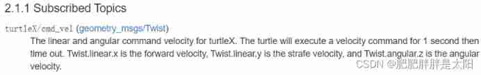
Demonstrate "topic communication, action communication, service communication and parameter server" with a small turtle case

Detailed explanation of memory addressing in 8086 real address mode
![[image denoising] image denoising based on nonlocal Euclidean median (nlem) with matlab code](/img/1e/386cf601f8f60197adbc853f321472.png)
[image denoising] image denoising based on nonlocal Euclidean median (nlem) with matlab code

Kali and programming: how to quickly build the OWASP website security test range?

Detailed explanation of 8086/8088 system bus (sequence analysis + bus related knowledge)
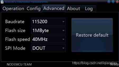
Esp8266 firmware upgrade method (esp8266-01s module)

ROS dynamic parameter configuration: use of dynparam command line tool (example + code)
"I was laid off by a big factory"

【图像去噪】基于高斯滤波、均值滤波、中值滤波、双边滤波四种滤波实现椒盐噪声图像去噪附matlab代码
随机推荐
D
tmux 和 vim 的快捷键修改
Problems encountered in learning go
2022年G3锅炉水处理复训题库及答案
leetcode. 39 --- combined sum
RT thread studio learning (I) new project
[data clustering] data set, visualization and precautions are involved in this column
6 functions
New knowledge: monkey improved app crawler
Decoupling in D
Jackson XML is directly converted to JSON without writing entity classes manually
Test left shift real introduction
Database syntax related problems, solve a correct syntax
企业微信官方 加解密库 PHP7版本报错 mcrypt_module_open 未定义方法 并且被PHP抛弃 解决方法使用 openssl解决
Expansion of D @nogc
Elegantly spliced XML
Use case design of software testing interview questions
C language sizeof strlen
【图像去噪】基于高斯滤波、均值滤波、中值滤波、双边滤波四种滤波实现椒盐噪声图像去噪附matlab代码
How to update kubernetes certificates