Statistical learning method (4/22) naive Bayes

Naive Bayes （naive bayes） Method is a classification method based on Bayesian theorem and the assumption of independence of feature conditions . For a given set of training data , Firstly, the joint probability distribution of input and output is learned based on the assumption of characteristic condition independence ： And then based on this model , For the given input x, Using Bayes theorem to get the output with the maximum posterior probability y. Naive Bayes is easy to implement , Efficient learning and forecasting , Is a common method .

Eye of depth course link ：https://ai.deepshare.net/detail/p_619b93d0e4b07ededa9fcca0/5
Code link ：
https://github.com/zxs-000202/Statistical-Learning-Methods

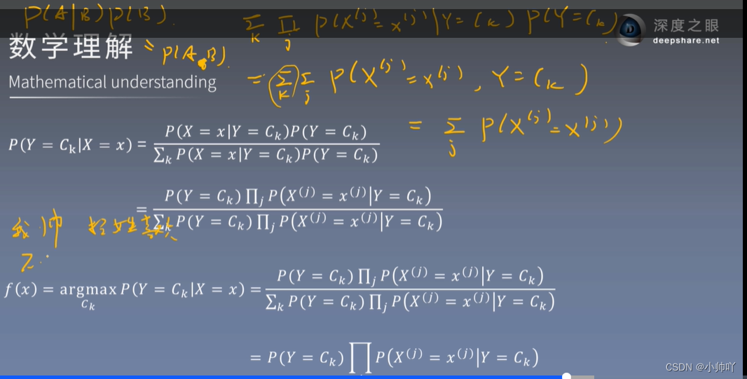
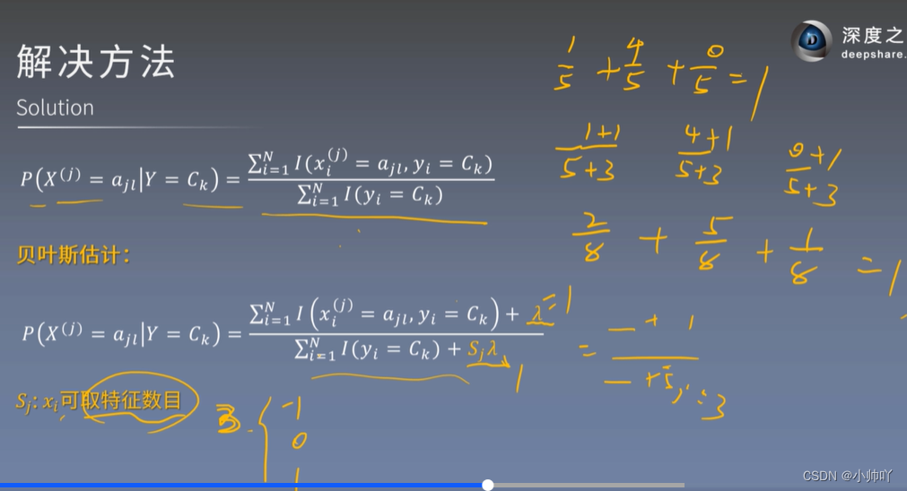
In the process of derivation, there will be a situation in which the number of samples is zero and the denominator is zero

A posteriori probability maximization is equivalent to expected risk minimization

# coding=utf-8
# Author:Dodo
# Date:2018-11-17
# Email:[email protected]

'''  Data sets ：Mnist  Number of training sets ：60000  Number of test sets ：10000 ------------------------------  Running results ：  Accuracy rate ：84.3%  Run time ：103s '''

import numpy as np
import time

def loadData(fileName):
    '''  Load the file  :param fileName: File path to load  :return:  Data sets and tag sets  '''
    # Store data and mark 
    dataArr = []; labelArr = []
    # Read the file 
    fr = open(fileName)
    # Traverse every line in the file 
    for line in fr.readlines():
        # Get current row , And press “,” Cut into fields and put them in the list 
        #strip： Remove the characters specified at the beginning and end of each line of string （ Default space or newline ）
        #split： Cut the string into each field according to the specified characters , Return to list form 
        curLine = line.strip().split(',')
        # Put the data in each row except the tag into the data set （curLine[0] Tag information for ）
        # At the same time, the data in the original string form is converted to integer 
        # In addition, the data is binarized , Greater than 128 Of into 1, Less than is converted to 0, Convenient for subsequent calculation 
        dataArr.append([int(int(num) > 128) for num in curLine[1:]])
        # Put tag information into the tag set 
        # Convert tag to integer while placing 
        labelArr.append(int(curLine[0]))
    # Return data sets and tags 
    return dataArr, labelArr

def NaiveBayes(Py, Px_y, x):
    '''  Probability estimation by naive Bayes  :param Py:  A priori probability distribution  :param Px_y:  Conditional probability distribution  :param x:  Sample to estimate x :return:  Back to all label The estimated probability of  '''
    # Set the number of features 
    featrueNum = 784
    # Set the number of categories 
    classNum = 10
    # Create an array of estimated probabilities to store all tags 
    P = [0] * classNum
    # For each category , Estimate the probability separately 
    for i in range(classNum):
        # initialization sum by 0,sum For the sum term .
        # In the training process, the probability is log Handle , So here we should have multiplied all the probabilities , Finally, compare which probability is the greatest 
        # But when used log When dealing with , Successive multiplication becomes accumulation , So use sum
        sum = 0
        # Get each conditional probability value , Add up 
        for j in range(featrueNum):
            sum += Px_y[i][j][x[j]]
        # And then add it to the prior probability （ That's the formula 4.7 A priori probability in times the later ones , Multiplication because log It all becomes addition ）
        P[i] = sum + Py[i]

    #max(P)： Find the maximum probability 
    #P.index(max(P))： Find all corresponding to the maximum value of the probability （ The index value is equal to the label value ）
    return P.index(max(P))


def model_test(Py, Px_y, testDataArr, testLabelArr):
    '''  Test the test set  :param Py:  A priori probability distribution  :param Px_y:  Conditional probability distribution  :param testDataArr:  Test set data  :param testLabelArr:  Test set tag  :return:  Accuracy rate  '''
    # Error value count 
    errorCnt = 0
    # Loop through each sample in the test set 
    for i in range(len(testDataArr)):
        # Get predictions 
        presict = NaiveBayes(Py, Px_y, testDataArr[i])
        # Compare with the answer 
        if presict != testLabelArr[i]:
            # If wrong   Error value count plus 1
            errorCnt += 1
    # Return accuracy 
    return 1 - (errorCnt / len(testDataArr))


def getAllProbability(trainDataArr, trainLabelArr):
    '''  The prior probability distribution and conditional probability distribution are calculated through the training set  :param trainDataArr:  Training data set  :param trainLabelArr:  Training tag set  :return:  Prior probability distribution and conditional probability distribution  '''
    # Set the number of special diagnosis samples , The handwritten pictures in the dataset are 28*28, The transformation to a vector is 784 dimension .
    # （ Our data set has been converted from images to 784 The form of dimension ,CSV In the format is ）
    featureNum = 784
    # Set the number of categories ,0-9 There are ten categories 
    classNum = 10

    # Initialize the prior probability distribution to store the array , The result of subsequent calculation P(Y = 0) Put it in Py[0] in , And so on 
    # The data length is 10 That's ok 1 Column 
    Py = np.zeros((classNum, 1))
    # Cycle through each category , Calculate their prior probability distributions respectively 
    # The calculation formula is "4.2 section   Parameter estimation of naive Bayesian method   The formula 4.8"
    for i in range(classNum):
        # The following formula is taken apart for analysis 
        #np.mat(trainLabelArr) == i： Convert labels to matrix form , Every one of them has something to do with i Compare , If equal , This bit becomes Ture, conversely False
        #np.sum(np.mat(trainLabelArr) == i): Calculate the matrix obtained in the previous step Ture The number of , In sum ( Intuitively, it is to find all label How many of them 
        # by i The tag , Get 4.8 type P（Y = Ck） The molecule in )
        #np.sum(np.mat(trainLabelArr) == i)) + 1： Reference resources “4.2.3 section   Bayesian estimation ”, For example, if the dataset does not exist y=1 The tag , in other words 
        # There are no... In the handwritten dataset 1 This picture , So if you don't add 1, Because there is no y=1, So the molecule becomes 0, So when we finally find the posterior probability, this term becomes 0, Again 
        # And conditional probability , The result is also 0, This is not allowed , So molecules add 1, Denominator plus K（K The number of values taken for the tag , Here you are 10 Number , The value is 10）
        # Refer to the formula 4.11
        #(len(trainLabelArr) + 10)： The total length of the label set +10.
        #((np.sum(np.mat(trainLabelArr) == i)) + 1) / (len(trainLabelArr) + 10)： A priori probability finally obtained 
        Py[i] = ((np.sum(np.mat(trainLabelArr) == i)) + 1) / (len(trainLabelArr) + 10)
    # Convert to log Logarithmic form 
    #log It is not written in the book , But in practice, we need to consider , And the reason is that ：
    # Finally, when we get the posterior probability estimation , Form is the multiplication of items （“4.1  Learning of naive Bayes method ”  type 4.7）, There are two problems ：1. A certain item is 0 when , The result is 0.
    # This problem can be eliminated by adding a corresponding number to the numerator and denominator , It has been handled well .2. If there are many special cases （ For example, here , The items that need to be connected are 784 Features 
    # Add a prior probability distribution to get a total of 795 Item multiplication , All numbers are 0-1 Between , The result must be a small approach 0 Number of numbers .） Theoretically, it can be judged by the size of the result ,  But in 
    # It is very likely that the program will overflow downward during operation and cannot be compared , Because the value is too small . Therefore, the value is artificially calculated log Handle .log It is an increasing function in the domain of definition , in other words log（x） in ,
    #x The bigger it is ,log And the bigger , Monotonicity is consistent with the original data . So add log It has no effect on the result . In addition, the multiplicative term passes log in the future , It can become the accumulation of items , Simplify the calculation .
    # In the likelihood function, we usually use log The way to deal with （ As for why this book does not cover , I don't know either ）
    Py = np.log(Py)

    # Calculate the conditional probability  Px_y=P（X=x|Y = y）
    # The calculation of conditional probability is divided into two steps , The first big one below for A loop is used to accumulate , In reference books “4.2.3  Bayesian estimation   type 4.10”, The first big one below for Inside the loop is 
    # Used to calculate 4.10 The molecules of , As for the molecular +1 And the calculation of denominator is the second largest below For Inside 
    # Initialize to full 0 matrix , Used to store conditional probabilities in all cases 
    Px_y = np.zeros((classNum, featureNum, 2))
    # Traverse the tag set 
    for i in range(len(trainLabelArr)):
        # Get the tag used by the current loop 
        label = trainLabelArr[i]
        # Get the current sample to be processed 
        x = trainDataArr[i]
        # Traverse each vitta of the sample 
        for j in range(featureNum):
            # Add... To the corresponding position in the matrix 1
            # The conditional probability has not been calculated here , First add up all the numbers , After adding it all , In the following steps, the corresponding conditional probability is calculated 
            Px_y[label][j][x[j]] += 1


    # The second big for, Calculation formula 4.10 Denominator of , And the division between numerator and denominator 
    # Loop through each tag （ common 10 individual ）
    for label in range(classNum):
        # Cycle each feature corresponding to each tag 
        for j in range(featureNum):
            # obtain y=label, The first j Special diagnosis 0 The number of 
            Px_y0 = Px_y[label][j][0]
            # obtain y=label, The first j Special diagnosis 1 The number of 
            Px_y1 = Px_y[label][j][1]
            # fitting 4.10 Divide the numerator and denominator of , Before division, it is based on Bayesian estimation , The denominator needs to be added with 2（ The number of values that can be taken for each feature ）
            # Calculate separately for y= label,x The first j The first characteristic is 0 and 1 Conditional probability distribution of 
            Px_y[label][j][0] = np.log((Px_y0 + 1) / (Px_y0 + Px_y1 + 2))
            Px_y[label][j][1] = np.log((Px_y1 + 1) / (Px_y0 + Px_y1 + 2))

    # Returns a priori probability distribution and conditional probability distribution 
    return Py, Px_y


if __name__ == "__main__":
    start = time.time()
    #  Get the training set 
    print('start read transSet')
    trainDataArr, trainLabelArr = loadData('../Mnist/mnist_train.csv')

    #  Get the test set 
    print('start read testSet')
    testDataArr, testLabelArr = loadData('../Mnist/mnist_test.csv')

    # Start training , Learn prior probability distribution and conditional probability distribution 
    print('start to train')
    Py, Px_y = getAllProbability(trainDataArr, trainLabelArr)

    # Test the test set using the learned prior probability distribution and conditional probability distribution 
    print('start to test')
    accuracy = model_test(Py, Px_y, testDataArr, testLabelArr)

    # Print accuracy 
    print('the accuracy is:', accuracy)
    # Print time 
    print('time span:', time.time() -start)