Reading notes of cgnf: conditional graph neural fields

One . An overview of the article

In most GNNs in , The dependency between node labels is not considered . So , The author puts the conditional random field （Conditional Random Fields, CRF） And graph convolution network CGNF（Conditional Graph Neural Network）, This model explicitly models the joint probability of the whole node label set , thus The neighborhood label information can be used in the node label prediction task .

Two . Background knowledge

2.1 Figure convolution network

GCN The mathematical form of convolution in the middle map is as follows ：
$${\mathbf{H}}^{(l+1)}=\sigma \left({\tilde{\mathbf{D}}}^{-\frac{1}{2}}\tilde{\mathbf{A}}{\tilde{\mathbf{D}}}^{-\frac{1}{2}}{\mathbf{H}}^{(l)}{\mathbf{W}}^{(l)}\right)$$
among $\tilde{A}=\mathbf{A}+\mathbf{I}$ Represents the adjacency matrix with self ring added ,$\tilde{D}$ yes $\tilde{A}$ The corresponding degree matrix （ Diagonal matrix ）,${\mathbf{H}}^{(l)}$ It means the first one $l$ The node representation of the layer ,${\mathbf{W}}^{(l)}$ It means the first one $l$ Layer weight matrix ,$\sigma$ Is the activation function , The common one is ReLU.

2.2 Conditional random field

Conditional random field （CRF） It's a kind of Undirected probability graph model , Usually used for structural prediction tasks . Given the input characteristics $x\in {\mathbb{R}}^d$,CRF To find the maximum conditional probability $P(\mathbf{y}\mid \mathbf{x})$ Tag set $\mathbf{y}$. On an undirected graph ,CRF The way to calculate the joint probability distribution is Factorization , namely ：
$$P(\mathbf{y}\mid \mathbf{x})=\frac{1}{Z(\mathbf{x})}\prod _c{\Phi }_a\left({\mathbf{x}}_c,{\mathbf{y}}_c\right)$$
among $c$ Represents the group in the figure ,${\mathbf{x}}_c$ Express Group $c$ Features corresponding to all vertices in ,${\Phi }_c$ Represents the potential function ,$Z(\mathbf{x})={\sum }_{{\mathbf{y}}_c^{\prime }}{\prod }_c{\Phi }_a\left({\mathbf{x}}_c,{\mathbf{y}}_c^{\prime }\right)$ Denotes the normalization factor （ It is used to ensure that the calculated probability value is legal ）.

Clique refers to a subgraph in which all vertices have edge connections .

3、 ... and .CGNF Detailed introduction

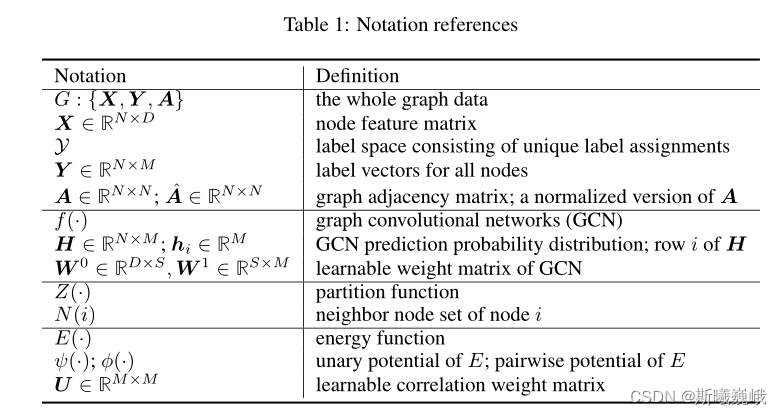
First, the symbol table is given for the convenience of subsequent introduction ：

3.1 Training

CGNF The first step is to input the graph $G=\{\mathbf{X},\mathbf{Y},\mathbf{A}\}$ Later Kipf and Welling Bring up the 2 layer GCN Model , namely ：
$$\mathbf{H}=f(\mathbf{X},\mathbf{A})=\mathrm{Softmax}\left(\hat{\mathbf{A}}\mathrm{ReLu}\left(\hat{\mathbf{A}}\mathbf{X}{\mathbf{W}}^0\right){\mathbf{W}}^1\right)$$
And then , The author considers the influence of node characteristics and label dependency , Define the energy function （energy function） as follows ：
$$E(\mathbf{Y},\mathbf{X},\mathbf{A})=E_c\left({\mathbf{Y}}_c,{\mathbf{X}}_c,\mathbf{A}\right)=\sum _i\psi \left({\mathbf{y}}_i,{\mathbf{x}}_i\right)+\gamma \sum _{(i,j)\in \mathcal{E},i<j}\varphi \left({\mathbf{y}}_i,{\mathbf{y}}_j,A_{i,j}\right)$$
among $c$ Express Group ,$\mathcal{E}$ Represents an edge set ,$\psi (\cdot )$ by The univariate potential function （ Used for policy observation nodes $x_i$ And labels $y_i$ Compatibility between compatibility, namely The observed value is $x_i$ Belong to $y_i$ The probability of a class ）, Pairwise potential function $\varphi (\cdot )$ Used to capture tag Correlation . Based on this energy function , Can export Gibbs Distribution ：
$$P(\mathbf{Y}\mid \mathbf{X},\mathbf{A})=\frac{\exp (-E(\mathbf{Y},\mathbf{X},\mathbf{A}))}{{\sum }_{{\mathbf{Y}}^{\prime }\in \mathcal{Y}}\exp \left(-E\left({\mathbf{Y}}^{\prime },\mathbf{X},\mathbf{A}\right)\right)}=\frac{\exp (-E(\mathbf{Y},\mathbf{X},\mathbf{A}))}{Z(\mathbf{X},\mathbf{A})}$$
The goal of the author is to maximize the conditional probability , namely ：
$$\begin{array}{rl}E(\mathbf{Y},\mathbf{X},\mathbf{A})& =\sum _i\psi \left({\mathbf{y}}_i,{\mathbf{h}}_{\mathbf{i}}\right)+\gamma \sum _{(i,j)\in \mathcal{E},i<j}\varphi \left({\mathbf{y}}_i,{\mathbf{y}}_j,{\hat{A}}_{i,j}\right)\\ & =\sum _i\left(\psi \left({\mathbf{y}}_i,{\mathbf{h}}_i\right)+\frac{\gamma }{2}\sum _{j\in N(i)}\varphi \left({\mathbf{y}}_i,{\mathbf{y}}_j,{\hat{A}}_{i,j}\right)\right)\end{array}$$
among $h_i$ It's through 2 layer GCN The node representation obtained by the model ,${\hat{A}}_{i,j}$ Is the original in the regularized adjacency matrix ,$N(i)$ Is the node $i$ The neighborhood of . The calculation formula of the two potential functions is as follows ：
$$\begin{array}{rl}\psi \left({\mathbf{y}}_i,{\mathbf{h}}_i\right)& =-\log p\left({\mathbf{y}}_i\mid {\mathbf{h}}_i\right)=-\sum _k{y}_{i,k}\log h_{i,k}\\ \varphi \left({\mathbf{y}}_i,{\mathbf{y}}_j,{\hat{A}}_{i,j}\right)& =-2{\hat{A}}_{i,j}{U}_{y_i,y_j}\end{array}$$
It can be seen from the above formula that $\psi \left({\mathbf{y}}_i,{\mathbf{h}}_i\right)$ It's actually cross entropy ,$U_{y_i,y_j}\in \mathbf{U}$ yes label $y_i$ and $y_j$ Learnable correlation weights between . Adopt a similar tradition CRF How to do it , The author uses negative log likelihood as the objective function of training ：
$$\begin{array}{rl}-\log P(\mathbf{Y}\mid \mathbf{X},\mathbf{A})& =E(\mathbf{Y},\mathbf{X},\mathbf{A})+\log Z(\mathbf{X},\mathbf{A})\\ & =E(\mathbf{Y},\mathbf{X},\mathbf{A})+\log \sum _{{\mathbf{Y}}^{\prime }}\exp \left(-E\left({\mathbf{Y}}^{\prime },\mathbf{X},\mathbf{A}\right)\right)\end{array}$$
In inferring （inference） When , just ${\min }_{\mathbf{Y}}E(\mathbf{Y},\mathbf{X},\mathbf{A})$ that will do . But it is more difficult to optimize than the above training objectives , For this reason, the author adopts Pseudo likelihood To approximate it ：
$$P(\mathbf{Y}\mid \mathbf{X},\mathbf{A})\approx PL(\mathbf{Y}\mid \mathbf{X},\mathbf{A})=\prod _{i}P\left({\mathbf{y}}_i\mid {\mathbf{y}}_{N(i)},\mathbf{X},\mathbf{A}\right)$$
among ：
$$\begin{array}{rl}P\left({\mathbf{y}}_i\mid {\mathbf{y}}_{N(i)},\mathbf{X},\mathbf{A}\right)& =\frac{\exp (-\psi \left({\mathbf{y}}_i,{\mathbf{h}}_{\mathbf{i}}\right)-\gamma {\sum }_{j\in N(i)}\varphi \left({\mathbf{y}}_i,{\mathbf{y}}_j,{\hat{A}}_{i,j}\right)}{{\sum }_{{\mathbf{y}}_i^{\prime }}(\exp \left(-\psi \left({\mathbf{y}}_i^{\prime },{\mathbf{h}}_{\mathbf{i}}\right)-\gamma {\sum }_{j\in N(i)}\varphi \left({\mathbf{y}}_i^{\prime },{\mathbf{y}}_j,{\hat{A}}_{i,j}\right)\right)}\\ & =\frac{\exp (-\log p\left({\mathbf{y}}_i\mid {\mathbf{h}}_{\mathbf{i}}\right)-2\gamma {\sum }_{j\in N(i)}{\hat{A}}_{i,j}{U}_{y_i,y_j}}{{\sum }_{{\mathbf{y}}_i^{\prime }}(\exp \left(-\log p\left({\mathbf{y}}_i^{\prime }\mid {\mathbf{h}}_{\mathbf{i}}\right)-2\gamma {\sum }_{j\in N(i)}{\hat{A}}_{i,j}{U}_{y_i^{\prime },y_j}\right)}\end{array}$$
${\mathbf{y}}_i^{\prime }$ Is the node ${\mathbf{x}}_i$ All possible labels . therefore , The new training goal is ：
$$\begin{array}{rl}& -\log PL(\mathbf{Y}\mid \mathbf{X},\mathbf{A})=\sum _i-\log P\left({\mathbf{y}}_i\mid {\mathbf{y}}_{N(i)},\mathbf{X},\mathbf{A}\right)=\\ & \sum _i(\psi \left({\mathbf{y}}_i,{\mathbf{h}}_i\right)+\gamma \sum _{j\in N(i)}\varphi \left({\mathbf{y}}_i,{\mathbf{y}}_j,{\hat{A}}_{i,j}\right)+\log \sum _{{\mathbf{y}}_i^{\prime }}\left(\exp \left(-\psi \left({\mathbf{y}}_i^{\prime },{\mathbf{h}}_{\mathbf{i}}\right)-\gamma \sum _{j\in N(i)}\varphi \left({\mathbf{y}}_i^{\prime },{\mathbf{y}}_j,{\hat{A}}_{i,j}\right)\right)\right)\\ & =-\sum _{i,k}(\mathbf{Y}\odot \log \mathbf{H}{)}_{i,k}-2\gamma \sum _{i,j,i\ne j}{\left(\hat{\mathbf{A}}\odot \left(\mathbf{Y}\mathbf{U}{\mathbf{Y}}^T\right)\right)}_{i,j}+\sum _i\log \sum _k(\mathbf{H}\odot \exp (2\gamma \hat{\mathbf{A}}\mathbf{Y}\mathbf{U}){)}_{i,k}\end{array}$$
$\odot$ Represents element by element multiplication .

3.2 infer

As mentioned above , When inferring, you only need to optimize the following objectives ：
$$\underset{{\hat{\mathbf{Y}}}_{te}}{\min }E\left({\hat{\mathbf{Y}}}_{te},\mathbf{X},\mathbf{A},{\mathbf{Y}}_{tr}\right)=\underset{{\hat{\mathbf{Y}}}_{te}}{\min }\left[-\log p\left({\hat{\mathbf{Y}}}_{te}\mid \mathbf{H}\right)-\gamma \sum _{i\ne j}{\left(\hat{\mathbf{A}}\odot \left(\hat{\mathbf{Y}}\mathbf{U}{\hat{\mathbf{Y}}}^T\right)\right)}_{i,j}\right]$$
among $\hat{\mathbf{Y}}=$ concatenate $\left({\mathbf{Y}}_{tr},{\hat{\mathbf{Y}}}_{te}\right)$. The author mentioned two inference methods in his paper .

3.2.1 Inference method 1

The simplest inference method is to ignore the correlation between tags , namely ：
$$y_i=\underset{y_j}{\mathrm{argmin}}E\left({\mathbf{y}}_i,{\mathbf{Y}}_{tr},\mathbf{X},\mathbf{A}\right)=\underset{j}{\mathrm{argmin}}{\left[-\log \left({\mathbf{h}}_i\right)-2\gamma {\hat{\mathbf{A}}}_{tr}\mathbf{Y}{\mathbf{U}}^T\right]}_j$$

3.2.2 Inference method 2

The second scheme is to use dynamic programming method to find the optimal value . This method will randomly select a test node as the start , And randomly sort other test nodes , Then follow the order of sorting test nodes beam search（beam The size is $K$, That is, you can get $K$ Best set ）. Repeat the process $T$ word , Then select the best of all search results , The algorithm is summarized as follows ：

Four . experiment

The author in Cora、Pubmed、Citeseer and PPI Experiment on four data sets , And compared with others baseline Good performance has been achieved , The corresponding results are as follows ：

Conclusion

Reference material ：

• Understand conditional random fields
• CRF Conditional random field