当前位置:网站首页>Pytorch Basics
Pytorch Basics
2022-07-02 05:29:00 【Star soul is not a dream】
1. The difference between dynamic graph and static graph ? What is automatic differentiation ?
2. course
https://pytorch.apachecn.org/#/docs/1.7/043
Building neural networks
- Define neural networks , Get one model
- Define the loss function : torch.nn.xxLoss
- Define optimizer , Construct a optimizer object : torch.optim.xx
Training neural network
- Positive communication
- Calculate according to the loss function loss
- Back propagation :loss.backward()
- gradient descent :optimizer.step()
- The gradient goes to zero :optimizer.zero_grad()
tensor
- Generating tensor
- torch.tensor(data)
- torch.from_numpy(np_array)
- torch.xx_like(data, dtype=torch.float) # rewrite data Data type of
- torch.xx(shape) Such as :torch.rand(shape)
- attribute
- tensor.shape、tensor.dtype、tensor.device
- operation (tensor = tensor.to('cuda') # tensor Import GPU Inside )
- Index and slice
- Splicing : torch.cat
- Multiply elements by element : *, Matrix multiplication :@
- inplace operation : Such as : tensor.add_ ( Provincial memory , But error prone )
- numpy <--> torch ( Total memory area , Change at the same time )
- The tensor is transformed into Numpy array: tensor.numpy()
- Numpy array The array is transformed into a tensor :torch.from_numpy(xx)
Automatic derivation (Autograd): PyTorch Automatic differential engine
loss = (prediction - labels).sum()
loss.backward() # backward pass
When we call on the error tensor .backward() when , Start backpropagation . then ,Autograd Will calculate for each model parameter gradient And its Stored in the of the parameter .grad attribute in .
optim.step() #gradient descent call .step() start-up gradient descent . Optimizer pass .grad The gradient stored in is used to adjust each parameter .
Creating a tensor requires deriving it :
a = torch.tensor([2., 3.], requires_grad=True)loss.backward() Two cases :
- if loss It's a vector :
external_grad = torch.tensor([1., 1.])
loss.backward(gradient=external_grad)
# gradient Is with the loss Tensors of the same shape , It said loss Gradient relative to itself , All are 1
2. if loss It's scalar :
loss.sum().backward()Calculation chart :
Concept : Directed acyclic graph . Like an inverted number . Here is the input tensor , The root is the output tensor .
problem 1: What is a dynamic graph ?
Every time .backward() After call , Automatically build new graphs . So we can ask python Like breakpoint debugging .
Even if only one input tensor has requires_grad=True, The output tensor of the operation Gradients will also be required .
.requires_grad = False : Freeze parameters , Used to fine tune the model .
torch.no_grad() The context manager in can freeze parameters .
x = torch.tensor([1], requires_grad=True)
with torch.no_grad():
    y = x * 2
y.requires_grad # False
@torch.no_grad()
def doubler(x):
    return x * 2
z = doubler(x)
z.requires_grad # False
neural network :torch.nn
Defining network :
class Net(nn.Module):
    def __init__(self):
        super(Net, self).__init__()
        #  Custom layer
        # self. Layer name  = ...

    def forward(self, x):
        #  operation
        return x

net = Net()
print(net)
Just define forward function , You can use autograd Automatically define for you backward function ( Calculate the gradient
The learnable parameters of the model are determined by net.parameters() return
torch.nn Only small batches are supported , Input of a single sample is not supported .
for example ,nn.Conv2d Will adopt (b,c,h,w) Of 4D tensor .
If there is only one sample , Just use input.unsqueeze(0) Add a fake batch size (1,c,h,w).
Loss function :nn.MSELoss
CV: torchvision Package has a :torchvision.datasets and torch.utils.data.DataLoader.
GPU Training
- net.to(device)
- inputs, labels = data[0].to(device), data[1].to(device)
Define a new Autograd function
By definition torch.autograd.Function Subclass and implementation of forward and backward Function to easily define your own Autograd Operator . then , We can call new by constructing an instance and calling it like a function Autograd Operator , And pass the tensor containing the input data .
class LegendrePolynomial3(torch.autograd.Function):

    """

    We can implement our own custom autograd Functions by subclassing

    torch.autograd.Function and implementing the forward and backward passes

    which operate on Tensors.

    """

    @staticmethod

    def forward(ctx, input):

        """

        In the forward pass we receive a Tensor containing the input and return

        a Tensor containing the output. ctx is a context object that can be used

        to stash information for backward computation. You can cache arbitrary

        objects for use in the backward pass using the ctx.save_for_backward method.

        """

        ctx.save_for_backward(input)

        return 0.5 * (5 * input ** 3 - 3 * input)


    @staticmethod

    def backward(ctx, grad_output):

        """

        In the backward pass we receive a Tensor containing the gradient of the loss

        with respect to the output, and we need to compute the gradient of the loss

        with respect to the input.

        """

        input, = ctx.saved_tensors

        return grad_output * 1.5 * (5 * input ** 2 - 1)
Use :
       P3 = LegendrePolynomial3.apply

       y_pred = a + b * P3(c + d * x)
You can use the regular Python Flow control to achieve circulation ( Such as for), And you can define forward Simply reuse the same parameters many times to achieve weight sharing
Use Dataset
TensorDataset Is a data set packing tensor . By defining the length and manner of the index , This also provides us with iterations along the first dimension of the tensor , Indexing and slicing methods .
from torch.utils.data import TensorDataset
train_ds = TensorDataset(x_train, y_train)
xb,yb = train_ds[i*bs : i*bs+bs]
Use DataLoader
DataLoader Responsible for batch management , DataLoader Make iterations easier .
from torch.utils.data import DataLoader

train_dl = DataLoader(train_ds, batch_size=bs)

for xb,yb in train_dl:

pred = model(xb)


#  Verification set

valid_ds = TensorDataset(x_valid, y_valid)

valid_dl = DataLoader(valid_ds, batch_size=bs * 2)
Always call before training model.train(), And call before reasoning model.eval(), Because such as nn.BatchNorm2d and nn.Dropout Such layers will use them , To ensure that these different stages of behavior are correct .
    model.eval()

    with torch.no_grad():

        valid_loss = sum(loss_func(model(xb), yb) for xb, yb in valid_dl)
establish fit() and get_data()
def loss_batch(model, loss_func, xb, yb, opt=None):

    loss = loss_func(model(xb), yb)

    if opt is not None:

        loss.backward()

        opt.step()

        opt.zero_grad()

return loss.item(), len(xb)


import numpy as np

def fit(epochs, model, loss_func, opt, train_dl, valid_dl):

    for epoch in range(epochs):

        model.train()

        for xb, yb in train_dl:

            loss_batch(model, loss_func, xb, yb, opt)

        model.eval()

        with torch.no_grad():

            losses, nums = zip(

                *[loss_batch(model, loss_func, xb, yb) for xb, yb in valid_dl]

            )

        val_loss = np.sum(np.multiply(losses, nums)) / np.sum(nums)

        print(epoch, val_loss)

def get_data(train_ds, valid_ds, bs):

    return (

        DataLoader(train_ds, batch_size=bs, shuffle=True),

        DataLoader(valid_ds, batch_size=bs * 2),

)

train_dl, valid_dl = get_data(train_ds, valid_ds, bs)

model, opt = get_model()

fit(epochs, model, loss_func, opt, train_dl, valid_dl)
nn.Sequential
Sequential Object runs each module contained in it in a sequential manner
From the given function definition Custom layer , And then use Sequential This layer can be used when defining the network .
1. Conv2d
CLASS torch.nn.Conv2d(in_channels, out_channels, kernel_size, stride=1, padding=0, dilation=1, groups=1, bias=True, padding_mode='zeros', device=None, dtype=None)
dilation: Default: 1
2. MaxPool2d
CLASS torch.nn.MaxPool2d(kernel_size, stride=None, padding=0, dilation=1, return_indices=False, ceil_mode=False)
边栏推荐
- Youth training camp -- database operation project
- h5跳小程序
- 6. Network - Foundation
- 黑马笔记---Set系列集合
- Global and Chinese market of hydrocyclone desander 2022-2028: Research Report on technology, participants, trends, market size and share
- Appnuim environment configuration and basic knowledge
- Fabric. JS background is not affected by viewport transformation
- LS1046nfs挂载文件系统
- Latest: the list of universities and disciplines for the second round of "double first-class" construction was announced
- 操作符详解
猜你喜欢
6.网络-基础
【技术随记-08】

操作符详解
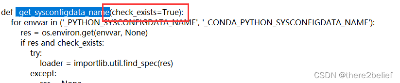
【pyinstaller】_get_sysconfigdata_name() missing 1 required positional argument: ‘check_exists‘
![Gee series: Unit 5 remote sensing image preprocessing [GEE grid preprocessing]](/img/1e/cf0aa09c2fce2278386f12eae4a6cd.jpg)
Gee series: Unit 5 remote sensing image preprocessing [GEE grid preprocessing]

Fabric.js 激活输入框
LeetCode 241. Design priorities for operational expressions (divide and conquer / mnemonic recursion / dynamic programming)
![Gee series: unit 7 remote sensing image classification using GEE [random forest classification]](/img/01/ba9441b7b1efaed85c464316740edb.jpg)
Gee series: unit 7 remote sensing image classification using GEE [random forest classification]

记录sentry的踩坑之路

LeetCode 1175. 质数排列(质数判断+组合数学)
随机推荐
来啦~ 使用 EasyExcel 导出时进行数据转换系列新篇章!
Essence and physical meaning of convolution (deep and brief understanding)
How matlab marks' a 'in the figure and how matlab marks points and solid points in the figure
摆正元素(带过渡动画)
Fabric.js 基础笔刷
Feign realizes file uploading and downloading
Get the details of the next largest number
Nodejs (03) -- custom module
Global and Chinese market of insulin pens 2022-2028: Research Report on technology, participants, trends, market size and share
黑马笔记---Set系列集合
Sliding window on the learning road
Usage record of vector
Gee: explore the change of water area in the North Canal basin over the past 30 years [year by year]
线程池概述
Fabric. JS compact JSON
Collectors.groupingBy 排序
Software testing learning - day 4
Black Horse Notes - - set Series Collection
Storage of data
el form 表单validate成功后没有执行逻辑