Three gradient descent methods and code implementation

Preface

This paper belongs to Linear regression algorithm 【AIoT Stage three 】（ Not updated yet ）, Here is an excerpt from one of them , It is convenient for readers to understand and read quickly according to their needs . This paper deduces through formula + Both aspects of the code are carried out at the same time , Because it involves compiling and running the code , If you don't $NumPy$,$Pandas$,$Matplotlib$ The basis of , It is suggested to fix the article first ： Data analysis three swordsmen 【AIoT Stage 1 （ Next ）】（ 100000 words blog post Nanny level explanation ）, This paper is the second part of gradient descent , Before learning, you need to learn ： gradient descent 【 Unconstrained optimization problems 】, There will be ： Gradient descent optimization , Gradient descent optimization advanced （ Update yet ）

1. Gradient descent method

1.1 The three gradients fall differently

There are three types of gradient descent ： Batch gradient descent $BGD$（Batch Gradient Descent）、 Small batch gradient descent $MBGD$（Mini-Batch Gradient Descent）、 Stochastic gradient descent $SGD$（Stochastic Gradient Descent）.

What is the difference between the three gradients ？ Let's start with the gradient descent step , The gradient descent step is divided into the following four steps ：

• 1、 Random assignment ,$Random$ Random number generation $\theta$, A random set of values $w_0、w_1\dots \dots w_n$

• 2、 Find gradient $g$ , The gradient represents the slope of the tangent at a point on the curve , Going down the tangent is equivalent to going down in the steepest direction of the slope

• 3、$if$$g<0$, $\theta$ Bigger ,$if$$g>0$, $\theta$ smaller

• 4、 Judge whether convergence or not $convergence$, If convergence jumps out of the iteration , If convergence is not achieved , Huidi $2$ Step perform... Again $2$ ~ $4$ Step

  The criterion of convergence is ： As the iteration progresses, the loss function $Loss$, The change is so small that it doesn't even change , That is, it is considered to reach convergence

The three gradients fall differently , Embodied in the second step ：

• $BGD$ It means in Every iteration Use All samples To update the gradient

• $MBGD$ It means in Every iteration Use Part of the sample （ All samples $500$ individual , Use among them $32$ Samples ） To update the gradient

• $SGD$ Refer to Every iteration Random selection A sample To do gradient update

1.2 Linear regression gradient update formula

Review the previous formula ！

The formula of the least square method is as follows ：

$J(\theta )=\frac{1}{2}\sum _{i=1}^n(h_{\theta }(x^{(i)})-y^{(i)}{)}^2$

Matrix writing ：

$J(\theta )=\frac{1}{2}(X\theta -y{)}^T(X\theta -y)$

Next, we will explain how to solve the problem of gradient descent $2$ Step , That is, we need to derive the derivative of the loss function to .

• ${\theta }_j^{n+1}={\theta }_j^n-\eta \ast \frac{\partial J(\theta )}{\partial {\theta }_j}$ among $j$ It means the first one $j$ A coefficient of

• $\frac{\partial J(\theta )}{\partial {\theta }_j}=\frac{\partial }{\partial {\theta }_j}\frac{1}{2}(h_{\theta }(x)-y{)}^2$

$=\frac{1}{2}\ast 2(h_{\theta }(x)-y)\frac{\partial }{\partial {\theta }_j}(h_{\theta }(x)-y)$$(1)$

$=(h_{\theta }(x)-y)\frac{\partial }{\partial {\theta }_j}(\sum _{i=0}^n{\theta }_i{x}_i-y)$$(2)$

$=(h_{\theta }(x)-y)x_j$$(3)$

  $x^2$ The derivative of is $2x$, According to the chain derivation rule , We can launch the first $(1)$ Step . Then multiple linear regression , therefore $h_{\theta }(x)$ Just yes ${\theta }^{T}x$ That is $w_0{x}_0+w_1{x}_1+\dots \dots +w_n{x}_n$ namely $\sum _{i=0}^n{\theta }_i{x}_i$. Here we are right ${\theta }_j$ To find the partial derivative , So and $w_j$ There is no negligible relationship , So there's only $x_j$.

   We can conclude that ${\theta }_j$ Corresponding gradient and predicted value $\hat{y}$ And real value $y$ of , here $\hat{y}$ and $y$ Is a column vector （ That is, multiple data ）, And also with ${\theta }_j$ Corresponding feature dimension $x_j$ of , here $x_j$ Is the second of the original dataset matrix $j$ Column . If we separate each dimension ${\theta }_0、{\theta }_1\dots \dots {\theta }_n$ Finding partial derivatives , The gradient values corresponding to all dimensions can be obtained .

• $g_0=(h_{\theta }(x)-y)x_0$
• $g_1=(h_{\theta }(x)-y)x_1$
• ……
• $g_j=(h_{\theta }(x)-y)x_j$

summary ：

${\theta }_j^{n+1}={\theta }_j^n-\eta \ast (h_{\theta }(x)-y)x_j$

1.3 Batch gradient descent $BGD$

Batch gradient descent method Is the most primitive form , It means in Every iteration Use All samples To update the gradient . The formula for updating parameters in each iteration is as follows ：

${\theta }_j^{n+1}={\theta }_j^n-\eta \ast \frac{1}{n}\sum _{i=1}^n(h_{\theta }(x^{(i)})-y^{(i)})x_j^{(i)}$

Get rid of $\frac{1}{n}$ It's fine too , Because it's a constant , You can talk to $\eta$ Merge

${\theta }_j^{n+1}={\theta }_j^n-\eta \ast \sum _{i=1}^n(h_{\theta }(x^{(i)})-y^{(i)})x_j^{(i)}$

Matrix writing ：

${\theta }^{n+1}={\theta }^n-\eta \ast X^T(X\theta -y)$

among $i=1,2,...,n$ Represents the number of samples , $j=0,1\dots \dots$ The number of features , Here we use the offset term , I.e. solution $x_0^{(i)}=1$.

Note that there is a summation function when updating here , That is to calculate and process all samples ！

advantage ：
  （1） One iteration is to compute all samples , At this point, the matrix is used to operate , Parallel .
  （2） The direction determined by the whole data set can better represent the sample population , So that we can be more accurate in the direction of the extremum . When the objective function is convex ,$BGD$ We must be able to get the global optimum .
shortcoming ：
  （1） When the number of samples $n$ When a large , Each iteration step needs to be calculated for all samples , The training process will be slow .

In terms of the number of iterations ,$BGD$ The number of iterations is relatively small . The convergence curve of its iteration can be shown as follows ：

1.4 Stochastic gradient descent $SGD$

Random gradient descent method Different from batch gradient descent , The random gradient descent is Every iteration Use A sample To update the parameters . Make training faster . The formula for updating parameters in each iteration is as follows ：

${\theta }_j^{n+1}={\theta }_j^n-\eta \ast (h_{\theta }(x^{(i)})-y^{(i)})x_j^{(i)}$

Batch gradient descent The algorithm will be used every time All The training sample , So these calculations are redundant , Because the same sample set is used every time . and Stochastic gradient descent The algorithm only selects randomly at a time One Samples to update model parameters , So every time you learn, you are very fast .

advantage ：
  （1） Because it is not an updated calculation on all training data , But in each iteration , Randomly select a piece of data for update calculation , In this way, the update speed of each round of parameters is greatly accelerated .
   shortcoming ：
  （1） Decreased accuracy . Because even if the objective function is strongly convex ,$SGD$ Still can't converge linearly .
  （2） It may converge to the local optimum , Because a single sample can't represent the trend of the whole sample .

Explain why SGD Convergence rate ratio BGD Be quick ：

• Here we assume that $30W$ Samples , about $BGD$ for , Each iteration requires calculation $30W$ Only samples can update the parameters once , It may take many iterations to get the minimum value （ So let's say that this is $10$）.
• And for $SGD$, Only one sample is required for each parameter update , So if you use this 30W Samples for parameter update , Then the parameters will be iterated $30W$ Time , And in the meantime ,$SGD$ It can ensure that it can converge to a suitable minimum .
• in other words , In convergence ,$BGD$ To calculate the $10\times 30W$ Time , and $SGD$ Only calculated $1\times 30W$ Time .

In terms of the number of iterations ,$SGD$ More iterations , The search process in solution space will be blind . The convergence curve of its iteration can be shown as follows ：

1.5 Small batch gradient descent $MBGD$

Small batch gradient descent , It is an example of batch gradient descent and random gradient descent compromise Way . The idea is ： Every iteration Use a portion of the total sample $(batc{h}_{s}ize)$ Samples to update parameters . So let's assume that $batc{h}_{s}ize=20$, Sample size $n=1000$ . The balance between update speed and update times is achieved . The formula for updating parameters in each iteration is as follows ：

${\theta }_j^{n+1}={\theta }_j^n-\eta \ast \frac{1}{batch\_size}\sum _{i=1}^{batch\_size}(h_{\theta }(x^{(i)})-y^{(i)})x_j^{(i)}$

Relative to random gradient descent algorithm , The small batch gradient descent algorithm reduces the convergence volatility , That is to say, the variance of parameter update is reduced , Make updates more stable . The gradient decreases relative to the total amount , It improves the speed of each learning . And it doesn't need to worry about the memory bottleneck, so it can use matrix operation to calculate efficiently .

In general , Small batch gradient descent is the recommended variant of gradient descent , Especially in deep learning . Choose... Randomly every time $2$ Idempotent number of samples to learn , for example ：$8$、$16$、$32$、$64$、$128$、$256$. Because the structure of computer is binary . But you have to choose according to the specific problem , Many tests can be carried out in practice , Select a number of samples with appropriate update speed and times .

$MBGD$ The convergence curve of gradient descent iteration is more gentle ：

2. Code implementation gradient descent

2.1 Batch gradient descent $BGD$

2.1.1 Univariate linear regression

import numpy as np

#  Create data 
X = np.random.rand(100, 1)
w, b = np.random.randint(1, 10, size = 2)
#  Increase noise , Also known as " Add salt "
y = w * X + b + np.random.rand(100, 1)
#  hold b As a bias term , Intercept correspondence coefficient  x_0 = 1,  to update  X
X = np.concatenate([X, np.full(shape = (100, 1), 
                               fill_value = 1)], axis = 1)

#  cycles 
epoches = 10000
#  Learning rate 
eta = 0.01
#  Coefficient of required solution ," Blind "
theta = np.random.randn(2, 1)

for i in range(epoches):
    #  Batch gradient descent ,X For matrix , Contains all the data 
    g = X.T.dot(X.dot(theta) - y)  #  The gradient calculated according to the formula 
    theta = theta - eta * g

print(' True slope 、 intercept ：', w, b)
print(' Use BGD Find the slope of 、 intercept ：', theta[0], theta[1])

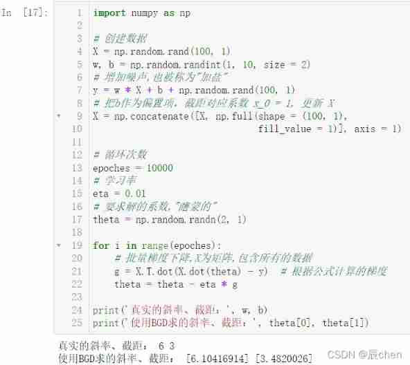
It can be seen that , There is still a certain gap between our calculated data and the real data , This is adding noise （ Add salt ） The result of the action of , But such calculation data is more real , Because data in real life cannot be perfect .

The following figure is a schematic diagram of gradient descent ：

We can see that , For the beginning of gradient descent ,$Learning$$step$ The larger , That is, the value of learning rate is relatively large , The closer you get to the right answer ,$Learning$$step$ The smaller it becomes , This actually gives us an idea , That our $eta$ It can change dynamically with the number of cycles that the gradient decreases ：

import numpy as np

#  Create data 
X = np.random.rand(100, 1)
w, b = np.random.randint(1, 10, size = 2)
#  Increase noise , Also known as " Add salt "
y = w * X + b + np.random.rand(100, 1)
#  hold b As a bias term , Intercept correspondence coefficient  x_0 = 1,  to update  X
X = np.concatenate([X, np.full(shape = (100, 1), 
                               fill_value = 1)], axis = 1)

#  cycles 
epoches = 10000

#  Learning rate 
t0, t1 = 5, 1000
# t  Is the number of gradient drops , Inverse time attenuation , As the gradient decreases, the number of times increases , The learning rate is getting smaller 
def learning_rate_shedule(t):
    return t0 / (t + t1)

#  Coefficient of required solution ," Blind "
theta = np.random.randn(2, 1)

for i in range(epoches):
    #  Batch gradient descent ,X For matrix , Contains all the data 
    g = X.T.dot(X.dot(theta) - y)  #  The gradient calculated according to the formula 
    eta = learning_rate_shedule(i)
    theta = theta - eta * g

print(' True slope 、 intercept ：', w, b)
print(' Use BGD Find the slope of 、 intercept ：', theta[0], theta[1])

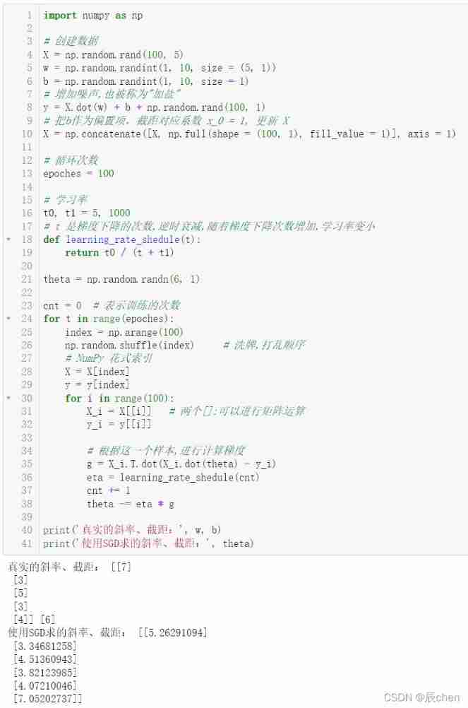
2.1.2 Eight variable linear regression

import numpy as np

#  Create data 
X = np.random.rand(100, 8)
w = np.random.randint(1, 10, size = (8, 1))
b = np.random.randint(1, 10, size = 1)

#  Increase noise , Also known as " Add salt "
y = X.dot(w) + b + np.random.rand(100, 1)
#  hold b As a bias term , Intercept correspondence coefficient  x_0 = 1,  to update  X
X = np.concatenate([X, np.full(shape = (100, 1), 
                               fill_value = 1)], axis = 1)

#  cycles 
epoches = 10000

#  Learning rate 
t0, t1 = 5, 1000
# t  Is the number of gradient drops , Inverse time attenuation , As the gradient decreases, the number of times increases , The learning rate is getting smaller 
def learning_rate_shedule(t):
    return t0 / (t + t1)

#  Coefficient of required solution ," Blind "
theta = np.random.randn(9, 1)

for i in range(epoches):
    #  Batch gradient descent ,X For matrix , Contains all the data 
    g = X.T.dot(X.dot(theta) - y)  #  The gradient calculated according to the formula 
    eta = learning_rate_shedule(i)
    theta = theta - eta * g

print(' True slope 、 intercept ：', w, b)
print(' Use BGD Find the slope of 、 intercept ：', theta)

2.2 Stochastic gradient descent $SGD$

2.2.1 Univariate linear regression

import numpy as np

#  Create data 
X = np.random.rand(100, 1)
w, b = np.random.randint(1, 10, size = 2)
#  Increase noise , Also known as " Add salt "
y = w * X + b + np.random.rand(100, 1)
#  hold b As a bias term , Intercept correspondence coefficient  x_0 = 1,  to update  X
X = np.concatenate([X, np.full_like(X, fill_value = 1)], axis = 1)

#  cycles 
epoches = 100

#  Learning rate 
t0, t1 = 5, 1000
# t  Is the number of gradient drops , Inverse time attenuation , As the gradient decreases, the number of times increases , The learning rate is getting smaller 
def learning_rate_shedule(t):
    return t0 / (t + t1)

theta = np.random.randn(2, 1)

cnt = 0  #  Indicates the number of workouts 
for t in range(epoches):
    index = np.arange(100)
    np.random.shuffle(index)     #  Shuffle , Out of order 
    # NumPy  Fancy index 
    X = X[index]
    y = y[index]
    for i in range(100):
        X_i = X[[i]]
        y_i = y[[i]]
        
        #  According to this sample , Calculate the gradient 
        g = X_i.T.dot(X_i.dot(theta) - y_i)
        eta = learning_rate_shedule(cnt)
        cnt += 1
        theta -= eta * g
        
print(' True slope 、 intercept ：', w, b)
print(' Use SGD Find the slope of 、 intercept ：', theta[0], theta[1])

2.2.2 Five variable linear regression

import numpy as np

#  Create data 
X = np.random.rand(100, 5)
w = np.random.randint(1, 10, size = (5, 1))
b = np.random.randint(1, 10, size = 1)
#  Increase noise , Also known as " Add salt "
y = X.dot(w) + b + np.random.rand(100, 1)
#  hold b As a bias term , Intercept correspondence coefficient  x_0 = 1,  to update  X
X = np.concatenate([X, np.full(shape = (100, 1), fill_value = 1)], axis = 1)

#  cycles 
epoches = 100

#  Learning rate 
t0, t1 = 5, 1000
# t  Is the number of gradient drops , Inverse time attenuation , As the gradient decreases, the number of times increases , The learning rate is getting smaller 
def learning_rate_shedule(t):
    return t0 / (t + t1)

theta = np.random.randn(6, 1)

cnt = 0  #  Indicates the number of workouts 
for t in range(epoches):
    index = np.arange(100)
    np.random.shuffle(index)     #  Shuffle , Out of order 
    # NumPy  Fancy index 
    X = X[index]
    y = y[index]
    for i in range(100):
        X_i = X[[i]]   #  Two []: You can do matrix operations 
        y_i = y[[i]]
        
        #  According to this sample , Calculate the gradient 
        g = X_i.T.dot(X_i.dot(theta) - y_i)
        eta = learning_rate_shedule(cnt)
        cnt += 1
        theta -= eta * g
        
print(' True slope 、 intercept ：', w, b)
print(' Use SGD Find the slope of 、 intercept ：', theta)

2.3 Small batch gradient descent $MBGD$

2.3.1 Univariate linear regression

import numpy as np

# 1、 Create a dataset X,y
X = np.random.rand(100, 1)
w,b = np.random.randint(1, 10,size = 2)
y = w * X + b + np.random.randn(100, 1)

# 2、 Use offset x_0 = 1, to update X
X = np.c_[X, np.ones((100, 1))]

# 3、 Define a function to adjust the learning rate 
t0, t1 = 5, 500
def learning_rate_schedule(t):
    return t0/(t + t1)

# 4、 Create a super parameter round 、 Number of samples 、 Small batch quantity 
epochs = 100
n = 100
batch_size = 16
num_batches = int(n / batch_size)

# 5、 initialization  W0...Wn, Standard Zhengtai distribution creates W
θ = np.random.randn(2, 1)

# 6、 many times for Loop to achieve gradient descent , The final result converges 
for epoch in range(epochs):
    #  On the double deck for Between cycles , Disrupt the data index order before each round starts the batch iteration 
    index = np.arange(n)
    np.random.shuffle(index)
    X = X[index]
    y = y[index]
    for i in range(num_batches):
        #  Take one batch of data at a time 16 Samples 
        X_batch = X[i * batch_size : (i + 1) * batch_size]
        y_batch = y[i * batch_size : (i + 1) * batch_size]
        g = X_batch.T.dot(X_batch.dot(θ) - y_batch)
        learning_rate = learning_rate_schedule(epoch * n + i)
        θ = θ - learning_rate * g

print(' The true slope and intercept are ：', w, b)
print(' The slope and intercept of gradient descent calculation are ：',θ)

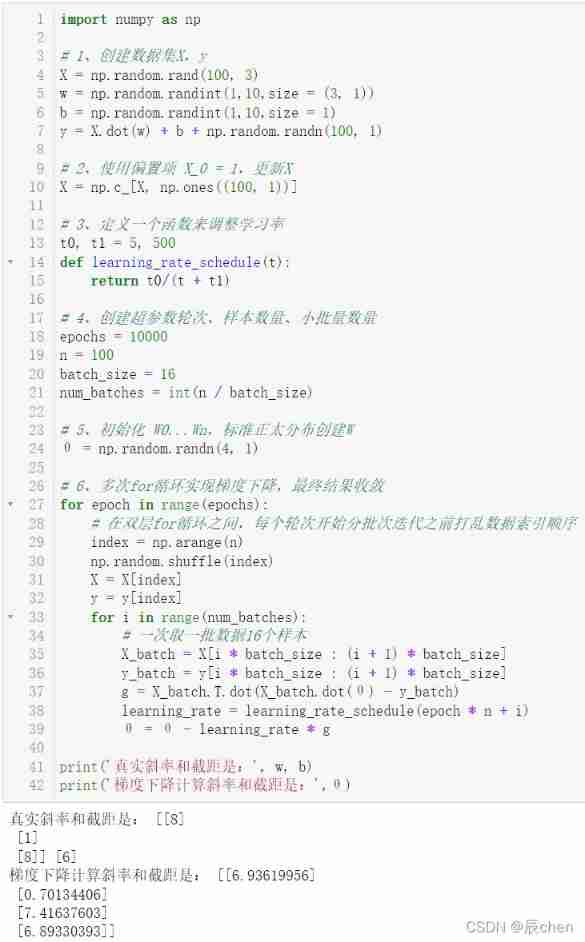
2.3.2 Ternary linear regression

import numpy as np

# 1、 Create a dataset X,y
X = np.random.rand(100, 3)
w = np.random.randint(1,10,size = (3, 1))
b = np.random.randint(1,10,size = 1)
y = X.dot(w) + b + np.random.randn(100, 1)

# 2、 Use offset  X_0 = 1, to update X
X = np.c_[X, np.ones((100, 1))]

# 3、 Define a function to adjust the learning rate 
t0, t1 = 5, 500
def learning_rate_schedule(t):
    return t0/(t + t1)

# 4、 Create a super parameter round 、 Number of samples 、 Small batch quantity 
epochs = 10000
n = 100
batch_size = 16
num_batches = int(n / batch_size)

# 5、 initialization  W0...Wn, Standard Zhengtai distribution creates W
θ = np.random.randn(4, 1)

# 6、 many times for Loop to achieve gradient descent , The final result converges 
for epoch in range(epochs):
    #  On the double deck for Between cycles , Disrupt the data index order before each round starts the batch iteration 
    index = np.arange(n)
    np.random.shuffle(index)
    X = X[index]
    y = y[index]
    for i in range(num_batches):
        #  Take one batch of data at a time 16 Samples 
        X_batch = X[i * batch_size : (i + 1) * batch_size]
        y_batch = y[i * batch_size : (i + 1) * batch_size]
        g = X_batch.T.dot(X_batch.dot(θ) - y_batch)
        learning_rate = learning_rate_schedule(epoch * n + i)
        θ = θ - learning_rate * g

print(' The true slope and intercept are ：', w, b)
print(' The slope and intercept of gradient descent calculation are ：',θ)