CNN flower classification

1、数据集介绍

总共5种花,According to the folder to distinguish the flowers in the category of the.

Download a package,You need to unpack it.

数据集下载地址：https://storage.googleapis.com/download.tensorflow.org/example_images/flower_photos.tgz

2、代码实战

2.1 导入依赖

import PIL
import numpy as np
import matplotlib.pyplot as plt
import pathlib
import lib

import tensorflow as tf
from tensorflow.keras import layers,models

2.2 下载数据

# 下载数据集到本地
data_url='https://storage.googleapis.com/download.tensorflow.org/example_images/flower_photos.tgz'
data_dir=tf.keras.utils.get_file('flower_photos',origin=data_url,untar=True)#untar=True 下载后解压
data_dir=pathlib.Path(data_dir)

2.3 统计数据集

# 统计数据集大小
dataset_size=len(list(data_dir.glob('*/*.jpg')))
dataset_size

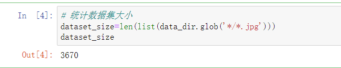
总共3670张照片,The puppy classification that much less than last time.

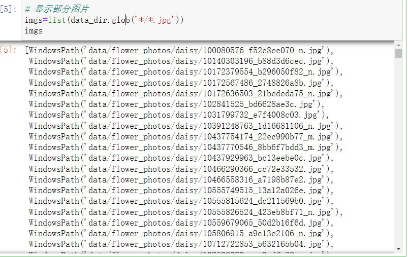
# 显示部分图片
imgs=list(data_dir.glob('*/*.jpg'))
imgs

Look at the first1张图片

img1=imgs[0] #第一张图片
img1

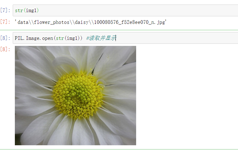
str(img1)

PIL.Image.open(str(img1)) #读取并显示

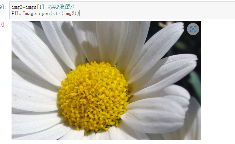
To view the world2张图片

img2=imgs[1] #第2张图片
PIL.Image.open(str(img2))

2.4 创建dataset

训练集：

# 3 创建dataset
BATCH_SIZE=32 
HEIGHT=180
WIDTH=180

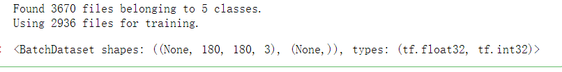
#80%是训练集,20%是验证集
train_ds=tf.keras.preprocessing.image_dataset_from_directory(directory=data_dir,
                                                            batch_size=BATCH_SIZE,
                                                            validation_split=0.2,
                                                            subset='training',
                                                            seed=666,
                                                            image_size=(HEIGHT,WIDTH))
train_ds

class_names=train_ds.class_names #数据集类别
class_names

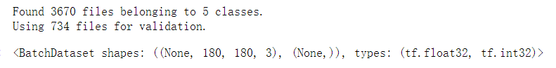
验证集：

val_ds=tf.keras.preprocessing.image_dataset_from_directory(directory=data_dir,
                                                            batch_size=BATCH_SIZE,
                                                            validation_split=0.2,
                                                            subset='validation',
                                                            seed=666,
                                                            image_size=(HEIGHT,WIDTH))
val_ds

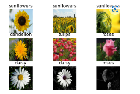
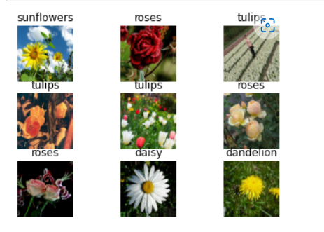
2.5 可视化一个batch_size

# 可视化一个batch_size的数据
for images,labels in train_ds.take(1):
    for i in range(9): # 一个batch_size有32张,这里只显示9张
        plt.subplot(3,3,i+1)
        plt.imshow(images[i].numpy().astype('uint8'))
        plt.title(class_names[labels[i]])
        plt.axis('off')

2.6 The data set into the in-memory cache,加速读取

#The data set into the in-memory cache,加速读取
AUTOTUNE=tf.data.AUTOTUNE
train_ds=train_ds.cache().shuffle(1000).prefetch(buffer_size=AUTOTUNE)
val_ds=val_ds.cache().prefetch(buffer_size=AUTOTUNE)

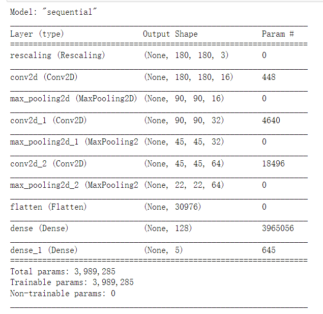
2.7 搭建模型

这里仅作测试,Does not use the training model

#搭建模型
model=models.Sequential([
    layers.experimental.preprocessing.Rescaling(1./255,input_shape=(HEIGHT,WIDTH,3)),# 数据归一化
    layers.Conv2D(16,3,padding='same',activation='relu'),
    layers.MaxPool2D(),
    layers.Conv2D(32,3,padding='same',activation='relu'),
    layers.MaxPool2D(),
    layers.Conv2D(64,3,padding='same',activation='relu'),
    layers.MaxPool2D(),
    layers.Flatten(),
    layers.Dense(128,activation='relu'),
    layers.Dense(5)
])

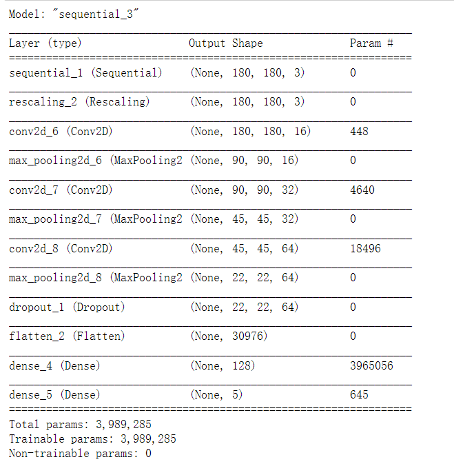
model.summary()

2.8 编译模型

#编译模型
model.compile(optimizer='adam',
             loss=tf.keras.losses.SparseCategoricalCrossentropy(from_logits=True),
             metrics=['accuracy'])

这里使用的SparseCategoricalCrossentropy会自动帮我们

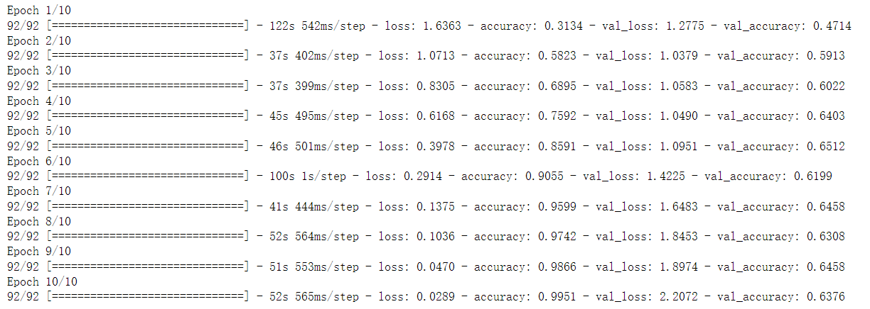
2.9 模型训练

#模型训练
EPOCHS=10
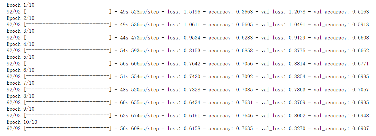
history=model.fit(train_ds,validation_data=val_ds,epochs=EPOCHS)

Pull across the equipment here is too,Slightly to have is a graphics card limit,So just set up10个epoch

2.10 可视化训练结果

# 可视化训练结果
ranges=range(EPOCHS)
train_acc=history.history['accuracy']
val_acc=history.history['val_accuracy']

train_loss=history.history['loss']
val_loss=history.history['val_loss']

plt.figure(figsize=(16,8))
plt.subplot(1,2,1)
plt.plot(ranges,train_acc,label='train_acc')
plt.plot(ranges,val_acc,label='val_acc')
plt.title('Accuracy')
plt.xlabel('Epochs')
plt.ylabel('Accuracy')

plt.subplot(1,2,2)
plt.plot(ranges,train_loss,label='train_loss')
plt.plot(ranges,val_loss,label='val_loss')
plt.title('Loss')
plt.xlabel('Epochs')
plt.ylabel('Loss')

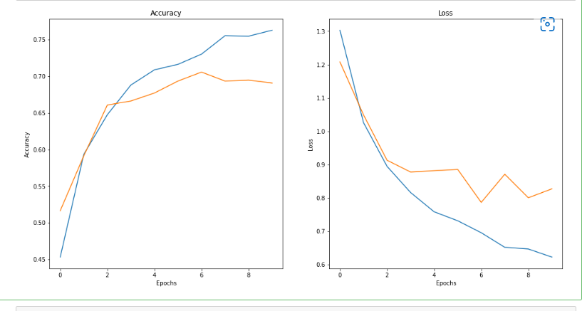
plt.show()

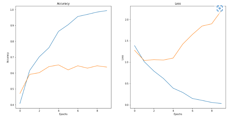
A fitting very serious,Below model is optimized

3、模型优化

3.1 Data to enhance Settings

# Data to enhance parameter Settings
data_argumentation=tf.keras.Sequential([
    # 随机水平翻转
    layers.experimental.preprocessing.RandomFlip('horizontal',input_shape=(HEIGHT,WIDTH,3)),
    # 随机旋转
    layers.experimental.preprocessing.RandomRotation(0.1), # 旋转
    # 随机缩放
    layers.experimental.preprocessing.RandomZoom(0.1),  # 
])

这块的API太多了,How to check the website.

3.2 The effect of display data enhanced

# The effect of display data enhanced
for images,labels in train_ds.take(1):
    for i in range(9): # 一个batch_size有32张,这里只显示9张
        plt.subplot(3,3,i+1)
        argumeng_images=data_argumentation(images) #数据增强
        plt.imshow(argumeng_images[i].numpy().astype('uint8')) # 显示
        plt.title(class_names[labels[i]])
        plt.axis('off')

3.3 搭建新的模型

#搭建新的模型
model_2=models.Sequential([
    data_argumentation, # 数据增强
    layers.experimental.preprocessing.Rescaling(1./255),# 数据归一化
    layers.Conv2D(16,3,padding='same',activation='relu'),
    layers.MaxPool2D(),
    layers.Conv2D(32,3,padding='same',activation='relu'),
    layers.MaxPool2D(),
    layers.Conv2D(64,3,padding='same',activation='relu'),
    layers.MaxPool2D(),
    layers.Dropout(0.2),
    layers.Flatten(),
    layers.Dense(128,activation='relu'),
    layers.Dense(5)
])

model_2.summary()

3.4 编译模型

#编译模型
model_2.compile(optimizer='adam',
             loss=tf.keras.losses.SparseCategoricalCrossentropy(from_logits=True),
             metrics=['accuracy'])

3.5 模型训练

#模型训练
history=model_2.fit(train_ds,validation_data=val_ds,epochs=EPOCHS)

3.6 可视化训练结果

# 可视化训练结果
ranges=range(EPOCHS)
train_acc=history.history['accuracy']
val_acc=history.history['val_accuracy']

train_loss=history.history['loss']
val_loss=history.history['val_loss']

plt.figure(figsize=(16,8))
plt.subplot(1,2,1)
plt.plot(ranges,train_acc,label='train_acc')
plt.plot(ranges,val_acc,label='val_acc')
plt.title('Accuracy')
plt.xlabel('Epochs')
plt.ylabel('Accuracy')

plt.subplot(1,2,2)
plt.plot(ranges,train_loss,label='train_loss')
plt.plot(ranges,val_loss,label='val_loss')
plt.title('Loss')
plt.xlabel('Epochs')
plt.ylabel('Loss')

plt.show()

Now, the effect is much better than before optimization.

3.7 模型预测

# 模型预测
test_img=tf.keras.preprocessing.image.load_img('sunfloor.jpg',target_size=(HEIGHT,WIDTH))
test_img

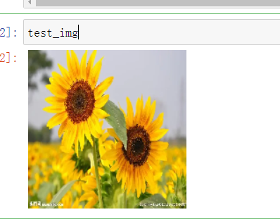
Here we ourselves on the Internet to download a picture of a sunflower forecast

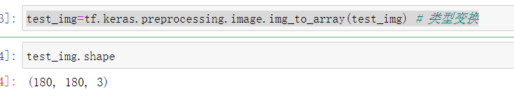
test_img=tf.keras.preprocessing.image.img_to_array(test_img) # 类型变换
test_img.shape

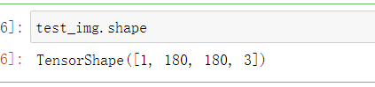
Expand the data d,Because the first dimension isbatchsize

test_img=tf.expand_dims(test_img,0) #扩充一维
test_img.shape

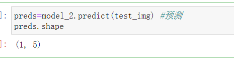
预测：

preds=model_2.predict(test_img) #预测
preds.shape

得分：

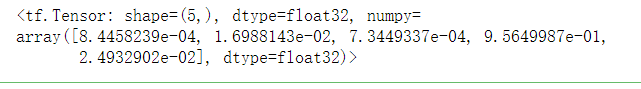
preds #得分

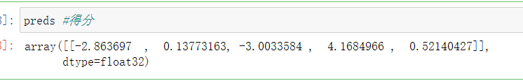
Score into probability：

scores=tf.nn.softmax(preds[0])# Score into probability
scores

print('Model to predict the most likely category is：{},概率值为：{}'.format(class_names[np.argmax(scores)],np.max(scores)))

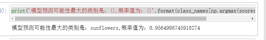
Here the last full connection layer can directly add asoftmax激活函数,After such predictions don't have to translate.