当前位置:网站首页>[point cloud processing paper crazy reading classic version 7] - dynamic edge conditioned filters in revolutionary neural networks on Graphs
[point cloud processing paper crazy reading classic version 7] - dynamic edge conditioned filters in revolutionary neural networks on Graphs
2022-07-03 09:08:00 【LingbinBu】
ECC: Dynamic boundary condition filter of graph convolution neural network
Abstract
- background : Many questions can be expressed based on graph Prediction of structural data
- Method : The convolution operation is extended from mesh to arbitrary graphs, At the same time, frequency domain , Can solve problems of different sizes and connectivity graph
- details : filters The weight of depends on the edge value from the vertex to the neighborhood ; Developed for graph Deep neural network for classification
- result : It works well in point cloud classification
- Code :https://github.com/mys007/ecc (PyTorch edition )
1. introduction
- A graph convolution neural network is constructed in the spatial domain ,filters The weight of depends on the value on the edge , And dynamically update each specific input . The proposed graph convolution network is suitable for any data structure
- The graph convolution network is applied to the point cloud classification task , And achieved better results
2. Related work
Frequency domain method
Spatial domain method
3. Method
3.1 Edge-Conditioned Convolution
Make l ∈ { 0 , . . , l max } l \in\left\{0, . ., l_{\max }\right\} l∈{ 0,..,lmax} Index for feedforward neural network layer .
Make G = G= G= ( V , E ) (V, E) (V,E) Represents an undirected or directed graph , among V V V Is the vertex. (Vertex) The finite set of ∣ V ∣ = n |V|=n ∣V∣=n, E ⊆ V × V E \subseteq V \times V E⊆V×V Is the edge (Edge) Set ∣ E ∣ = m |E|=m ∣E∣=m.
Suppose the graph is represented by vertices and edges , namely X l : V ↦ R d l X^{l}: V \mapsto \mathbb{R}^{d_{l}} Xl:V↦Rdl Indicates that each vertex is assigned a value (feature), L : E ↦ R s L: E \mapsto \mathbb{R}^{s} L:E↦Rs Indicates that each edge is assigned a value (attribute). All vertices can be represented in matrix form X l ∈ R n × d l X^{l} \in \mathbb{R}^{n \times d_{l}} Xl∈Rn×dl And all the edges L ∈ R m × s , X 0 L \in \mathbb{R}^{m \times s}, X^{0} L∈Rm×s,X0 Expressed as input signal .
The vertices i i i Of neighborhood N ( i ) = { j ; ( j , i ) ∈ E } ∪ { i } N(i)=\{j ;(j, i) \in E\} \cup\{i\} N(i)={ j;(j,i)∈E}∪{ i} Contains all adjacent vertices and i i i In itself .
The vertices i i i Situated filtered The signal X l ( i ) ∈ R d l X^{l}(i) \in \mathbb{R}^{d_{l}} Xl(i)∈Rdl Through its neighborhood Point signal X l − 1 ( j ) ∈ R d l − 1 X^{l-1}(j) \in \mathbb{R}^{d_{l-1}} Xl−1(j)∈Rdl−1, j ∈ N ( i ) j \in N(i) j∈N(i) The weighted sum of .
Although this way of exchange aggregation solves permutation-invariant and neighborhood The problem of variable size , But this also erases arbitrary structural information .( It means that the method of aggregation is too violent ? Updating with only vertices will lose structural information , So the boundary value is introduced as the weight )
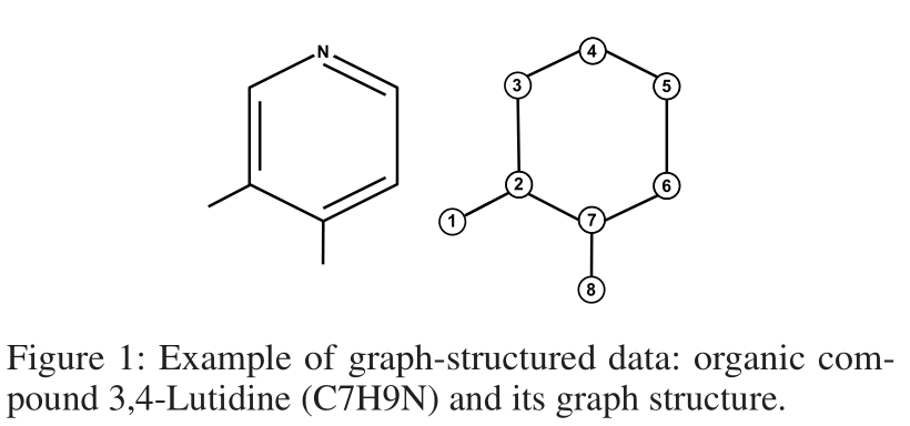
To solve this problem , It is proposed to add filter Condition of weight . Define an input as a boundary value L ( j , i ) L(j, i) L(j,i) Of filter-generating network F l : R s ↦ R d l × d l − 1 F^{l}: \mathbb{R}^{s} \mapsto \mathbb{R}^{d_{l} \times d_{l-1}} Fl:Rs↦Rdl×dl−1, The output is the weight matrix of a specific edge Θ j i l ∈ R d l × d l − 1 \Theta_{j i}^{l} \in \mathbb{R}^{d_{l} \times d_{l-1}} Θjil∈Rdl×dl−1, See the picture 1.
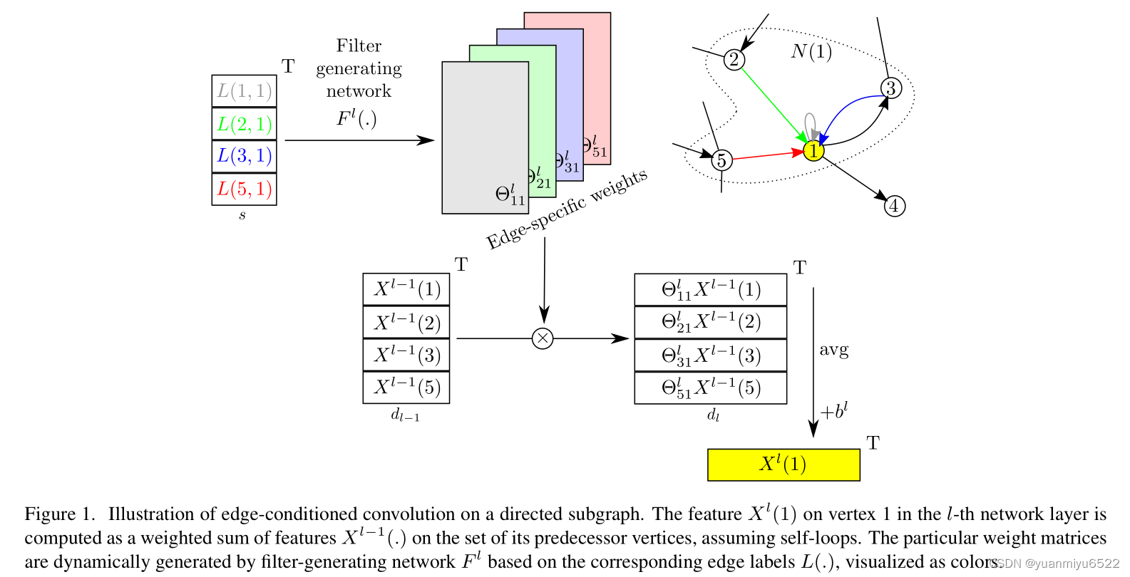
This is called Edge-Conditioned Convolution (ECC) Convolution operation of , It can be expressed as :
X l ( i ) = 1 ∣ N ( i ) ∣ ∑ j ∈ N ( i ) F l ( L ( j , i ) ; w l ) X l − 1 ( j ) + b l = 1 ∣ N ( i ) ∣ ∑ j ∈ N ( i ) Θ j i l X l − 1 ( j ) + b l \begin{aligned} X^{l}(i) &=\frac{1}{|N(i)|} \sum_{j \in N(i)} F^{l}\left(L(j, i) ; w^{l}\right) X^{l-1}(j)+b^{l} \\ &=\frac{1}{|N(i)|} \sum_{j \in N(i)} \Theta_{j i}^{l} X^{l-1}(j)+b^{l} \end{aligned} Xl(i)=∣N(i)∣1j∈N(i)∑Fl(L(j,i);wl)Xl−1(j)+bl=∣N(i)∣1j∈N(i)∑ΘjilXl−1(j)+bl
among b l ∈ R d l b^{l} \in \mathbb{R}^{d_{l}} bl∈Rdl Is a learnable bias , F l F^{l} Fl The learnable parameter of is the network weight w l w^{l} wl. w l w^{l} wl and b l b^{l} bl Is the model parameter , Update only during training , Θ j i l \Theta_{j i}^{l} Θjil Is based on input graph Parameters generated dynamically by the boundary value of .filter-generating network F l F^{l} Fl It can be any derivable model , This paper uses a multi-layer perceptron .
Complexity
Calculate for all vertices X l X^l Xl At most m m m Time F l F^l Fl The evaluation of , as well as m + n m+n m+n( Directed graph ) or 2 m + n 2m+n 2m+n( Undirected graph ) Submatrix - Vector multiplication . But in GPU It will be more efficient to operate on .
3.2 Relationship to Existing Formulations
Convolution on a regular grid can be seen as ECC A special form of .

3.3. Deep Networks with ECC
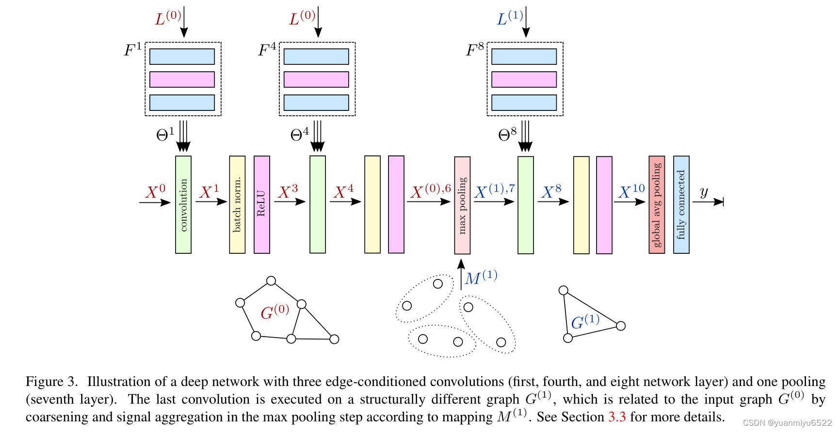
The network structure includes interleaved convolution 、 Global pooling and full connection layer , See the picture 3. In this way , The information obtained from the local neighborhood will be combined layer by layer to get the final context( Increase the acceptance domain ). Although the boundary value is specific graph It's fixed , But through filter generating networks the ( Study of the ) explain , It may change from one floor to another ( Not shared between layers F l F^l Fl The weight of ). therefore , Only 1-hop neighborhoods The limit ECC Will not be constrained , Similar to the standard CNN Use small 3×3filter In exchange for a deeper network , It's good .
Use after each convolution Batch Normalization, For fast convergence .
Pooling
Even though (non-strided) Convolution layer and all point-wise Layers do not change the foundation graph, And the signal can only be updated on the vertex , But the pooling layer is defined in a new 、coarsened graph Output aggregate signal on the vertex of . therefore , Must be entered for each graph Construct a step by step coarser Of graph h m a x h_{max} hmax Of pyramid.
Make h ∈ { 0 , … , h max } h \in\left\{0, \ldots, h_{\max }\right\} h∈{ 0,…,hmax} Express pyramid Different from graph G ( h ) = ( V ( h ) , E ( h ) ) G^{(h)}=\left(V^{(h)}, E^{(h)}\right) G(h)=(V(h),E(h)), every last G ( h ) G^{(h)} G(h) Both with L ( h ) L^{(h)} L(h) and X ( h ) , l X^{(h), l} X(h),l Related to .coarsening The process of includes 3 Step :
- subsampling or merging vertices
- creating the new edge structure E ( h ) E^{(h)} E(h) and labeling L ( h ) L^{(h)} L(h) (so-called reduction)
- mapping the vertices in the original graph to those in the coarsened one with M ( h ) : V ( h − 1 ) ↦ V ( h ) M^{(h)}: V^{(h-1)} \mapsto V^{(h)} M(h):V(h−1)↦V(h)
Final , The index for l h l_{h} lh The pooling layer of will X ( h − 1 ) , l h − 1 X^{(h-1), l_{h-1}} X(h−1),lh−1 Aggregate to be based on M ( h ) M^{(h)} M(h) Lower dimension of X ( h ) , l h X^{(h), l_{h}} X(h),lh.
stay coarsening In the process of , because self-edge Often appear , Therefore, there will be smaller graph Reduce to several disconnected vertices , There will be no problem . Because this structure is used to deal with variables n , m n,m n,m Of graph, We pass the overall situation average/max Pool operation solves the problem of graph The number of vertices of the change n h m a x n^{h_{max}} nhmax.
3.4. Application in Point Clouds
Graph Construction
Given a set of point clouds P P P And corresponding point features X P X_{P} XP, We construct a directed graph G = ( V , E ) G=(V, E) G=(V,E), And assign X 0 X^{0} X0 and L L L.
- For each point p ∈ P p \in P p∈P All construct vertices i ∈ V i \in V i∈V, adopt X 0 ( i ) = X P ( p ) X^{0}(i)=X_{P}(p) X0(i)=XP(p) Assign the corresponding signal ( If there are no features , Then the assignment is 0)
- Through the directed edge ( j , i ) (j, i) (j,i) Connect each vertex i i i And in space neighborhood The summit of j j j , Experiments show that ,Ball query Better
- In Cartesian and spherical coordinates ,6D vector L ( j , i ) = ( δ x , δ y , δ z , ∥ δ ∥ , arccos δ z / ∥ δ ∥ , arctan δ y / δ x ) L(j, i)=\left(\delta_{x}, \delta_{y}, \delta_{z},\|\delta\|, \arccos \delta_{z} /\|\delta\|, \arctan \delta_{y} / \delta_{x}\right) L(j,i)=(δx,δy,δz,∥δ∥,arccosδz/∥δ∥,arctanδy/δx) As the value on the edge , among δ = p j − p i \delta=p_{j}-p_{i} δ=pj−pi It means a vertex j , i j,i j,i Offset between .
Graph Coarsening
For a set of input point clouds P P P, adopt VoxelGrid algorithm Get the lower sampling point cloud pyramid P ( h ) P^{(h)} P(h), The specific process includes covering the point cloud with a resolution of r ( h ) r^{(h)} r(h) The grid of , For each voxel The point in takes the center of mass . Point cloud after each down sampling P ( h ) P^{(h)} P(h) Are independently transformed into neighborhood The radius is ρ ( h ) \rho^{(h)} ρ(h) Of graph G ( h ) G^{(h)} G(h) and labeling L ( h ) L^{(h)} L(h). Definition pooling map M ( h ) M^{(h)} M(h), Guarantee P ( h − 1 ) P^{(h-1)} P(h−1) Each point in is assigned to the lower sampling point cloud P ( h ) P^{(h)} P(h) In the middle distance ( P ( h − 1 ) P^{(h-1)} P(h−1) Every point in ) Some recent .
Data Augmentation
We randomly rotate point clouds about their upaxis, jitter their scale, perform mirroring, or delete random points.
4. experiment
C ( c ) \mathrm{C}(c) C(c) Express ECC The number of output channels is c c c, Follow behind batch normalization and ReLU Activation function . M P ( r , ρ ) \mathrm{MP}(r, \rho) MP(r,ρ) Represents the maximum pool layer ,grid A resolution of r r r,neighborhood The radius is ρ \rho ρ. G A P \mathrm{GAP} GAP Is the average pool layer . F C ( c ) \mathrm{FC}(c) FC(c) Is the number of channels c c c The full connection layer of . D ( p ) \mathrm{D}(p) D(p) Indicates that the probability is p p p Of dropouot.
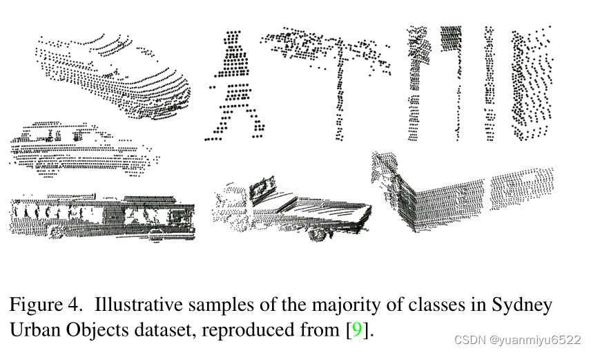
4.1 Sydney Urban Objects
C ( 16 ) − C ( 32 ) − M P ( 0.25 , 0.5 ) − C ( 32 ) − C ( 32 ) − M P ( 0.75 , 1.5 ) − C ( 64 ) − M P ( 1.5 , 1.5 ) − G A P − F C ( 64 ) − D ( 0.2 ) − F C ( 14 ) C(16)-C(32)-MP(0.25,0.5)-C(32)-C(32)-MP(0.75,1.5)-C(64)-MP(1.5,1.5)-GAP-FC(64)-D(0.2)-FC(14) C(16)−C(32)−MP(0.25,0.5)−C(32)−C(32)−MP(0.75,1.5)−C(64)−MP(1.5,1.5)−GAP−FC(64)−D(0.2)−FC(14)
C C C Inside F l F^l Fl contain F C ( 16 ) − F C ( 32 ) − F C ( d l d l − 1 ) FC(16)-FC(32)-FC(d_ld_{l−1}) FC(16)−FC(32)−FC(dldl−1)

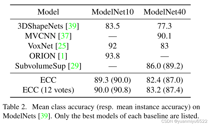
4.2 ModelNet
C ( 16 ) − C ( 32 ) − M P ( 2.5 / 32 , 7.5 / 32 ) − C ( 32 ) − C ( 32 ) − M P ( 7.5 / 32 , 22.5 / 32 ) − C ( 64 ) − G A P − F C ( 64 ) − D ( 0.2 ) − F C ( 10 ) C(16)-C(32)-MP(2.5/32,7.5/32)-C(32)-C(32)-MP(7.5/32,22.5/32)-C(64)-GAP-FC(64)-D(0.2)-FC(10) C(16)−C(32)−MP(2.5/32,7.5/32)−C(32)−C(32)−MP(7.5/32,22.5/32)−C(64)−GAP−FC(64)−D(0.2)−FC(10)
C C C Inside F l F^l Fl contain F C ( 16 ) − F C ( 32 ) − F C ( d l d l − 1 ) FC(16)-FC(32)-FC(d_ld_{l−1}) FC(16)−FC(32)−FC(dldl−1)
New words
- commutative adj. Exchangeable
- interlace v. Interlace , staggered
边栏推荐
- 精彩回顾|I/O Extended 2022 活动干货分享
- Recommend a low code open source project of yyds
- dried food! What problems will the intelligent management of retail industry encounter? It is enough to understand this article
- Mortgage Calculator
- Excel is not as good as jnpf form for 3 minutes in an hour. Leaders must praise it when making reports like this!
- Binary tree sorting (C language, char type)
- LeetCode 324. Swing sort II
- The method of replacing the newline character '\n' of a file with a space in the shell
- Binary tree sorting (C language, int type)
- AcWing 785. 快速排序(模板)
猜你喜欢
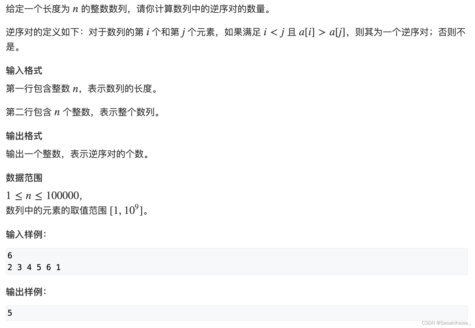
AcWing 788. Number of pairs in reverse order

数字化管理中台+低代码,JNPF开启企业数字化转型的新引擎

Notes and bugs generated during the use of h:i:s and y-m-d
【点云处理之论文狂读经典版13】—— Adaptive Graph Convolutional Neural Networks

In the digital transformation, what problems will occur in enterprise equipment management? Jnpf may be the "optimal solution"
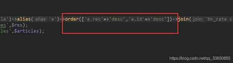
TP5 multi condition sorting

Education informatization has stepped into 2.0. How can jnpf help teachers reduce their burden and improve efficiency?

LeetCode 508. 出现次数最多的子树元素和
We have a common name, XX Gong

传统企业数字化转型需要经过哪几个阶段?
随机推荐
LeetCode 515. Find the maximum value in each tree row
What is the difference between sudo apt install and sudo apt -get install?
LeetCode 1089. 复写零
22-06-28 Xi'an redis (02) persistence mechanism, entry, transaction control, master-slave replication mechanism
With low code prospect, jnpf is flexible and easy to use, and uses intelligence to define a new office mode
拯救剧荒,程序员最爱看的高分美剧TOP10
Binary tree sorting (C language, char type)
Summary of methods for counting the number of file lines in shell scripts
Common penetration test range
I made mistakes that junior programmers all over the world would make, and I also made mistakes that I shouldn't have made
file_ put_ contents
LeetCode 508. The most frequent subtree elements and
TP5 multi condition sorting
too many open files解决方案
<, < <,>, > > Introduction in shell
LeetCode 324. 摆动排序 II
LeetCode 241. Design priorities for operational expressions
Log4j2 vulnerability recurrence and analysis
Recommend a low code open source project of yyds
State compression DP acwing 91 Shortest Hamilton path