当前位置:网站首页>【 YOLOv3中Loss部分计算】
【 YOLOv3中Loss部分计算】
2022-07-05 11:34:00 【网络星空(luoc)】
YOLOv1是一个anchor-free的,从YOLOv2开始引入了Anchor,在VOC2007数据集上将mAP提升了10个百分点。YOLOv3也继续使用了Anchor,本文主要讲ultralytics版YOLOv3的Loss部分的计算, 实际上这部分loss和原版差距非常大,并且可以通过arc指定loss的构建方式, 如果想看原版的loss可以在下方release的v6中下载源码。
Github地址: https://github.com/ultralytics/yolov3
Github release: https://github.com/ultralytics/yolov3/releases
1. Anchor
Faster R-CNN中Anchor的大小和比例是由人手工设计的,可能并不贴合数据集,有可能会给模型性能带来负面影响。YOLOv2和YOLOv3则是通过聚类算法得到最适合的k个框。聚类距离是通过IoU来定义,IoU越大,边框距离越近。
d(box,centroid)=1−IoU(box,centroid)
Anchor越多,平均IoU会越大,效果越好,但是会带来计算量上的负担,下图是YOLOv2论文中的聚类数量和平均IoU的关系图,在YOLOv2中选择了5个anchor作为精度和速度的平衡。
YOLOv2中聚类Anchor数量和IoU的关系图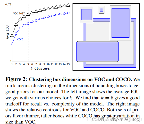
2. 偏移公式
在Faster RCNN中,中心坐标的偏移公式是:
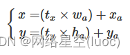
其中xa、ya 代表中心坐标,wa和ha代表宽和高,tx和ty
是模型预测的Anchor相对于Ground Truth的偏移量,通过计算得到的x,y就是最终预测框的中心坐标。
而在YOLOv2和YOLOv3中,对偏移量进行了限制,如果不限制偏移量,那么边框的中心可以在图像任何位置,可能导致训练的不稳定。

公式对应的意义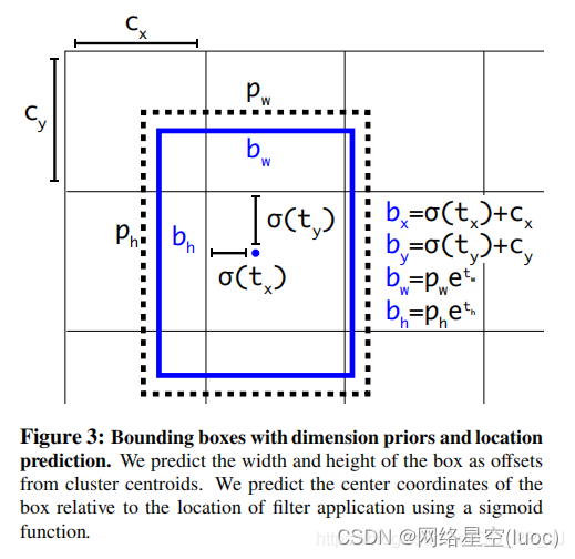
对照上图进行理解:
cx和cy分别代表中心点所处区域的左上角坐标。
pw和ph分别代表Anchor的宽和高。
σ(tx)和σ(ty)分别代表预测框中心点和左上角的距离,σ代表sigmoid函数,将偏移量限制在当前grid中,有利于模型收敛。
tw和th代表预测的宽高偏移量,Anchor的宽和高乘上指数化后的宽高,对Anchor的长宽进行调整。
σ(to)是置信度预测值,是当前框有目标的概率乘以bounding box和ground truth的IoU的结果
3. Loss
YOLOv3中有一个参数是ignore_thresh,在ultralytics版版的YOLOv3中对应的是train.py文件中的iou_t参数(默认为0.225)。
正负样本是按照以下规则决定的:
如果一个预测框与所有的Ground Truth的最大IoU<ignore_thresh时,那这个预测框就是负样本。
如果Ground Truth的中心点落在一个区域中,该区域就负责检测该物体。将与该物体有最大IoU的预测框作为正样本(注意这里没有用到ignore thresh,即使该最大IoU<ignore thresh也不会影响该预测框为正样本)
在YOLOv3中,Loss分为三个部分:
- 一个是xywh部分带来的误差,也就是bbox带来的loss
- 一个是置信度带来的误差,也就是obj带来的loss
- 最后一个是类别带来的误差,也就是class带来的loss
在代码中分别对应lbox, lobj, lcls,yolov3中使用的loss公式如下:
![lboxlclslobjloss=λcoord∑i=0S2∑j=0B1obji,j(2−wi×hi)[(xi−xi)2+(yi−yi)2+(wi−wi)2+(hi−hi)2]=λclass∑i=0S2∑j=0B1obji,j∑c∈classespi(c)log(pi(c))=λnoobj∑i=0S2∑j=0B1noobji,j(ci−ci)2+λobj∑i=0S2∑j=0B1obji,j(ci−ci^)2=lbox+lobj+lcls](/img/8c/1ad99b8fc1c5490f70dc81e1e5c27e.png)
其中:
S: 代表grid size, S2代表13x13,26x26, 52x52
B: box
1obj i,j: 如果在i,j处的box有目标,其值为1,否则为0
1noobj i,j: 如果在i,j处的box没有目标,其值为1,否则为0
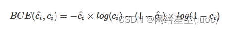
BCE(binary cross entropy)具体计算公式如下:
以上是论文中yolov3对应的darknet。而pytorch版本的yolov3改动比较大,有较大的改动空间,可以通过参数进行调整。
分成三个部分进行具体分析:
1. lbox部分
在ultralytics版版的YOLOv3中,使用的是GIOU,具体讲解见GIOU讲解链接。
简单来说是这样的公式,IoU公式如下:
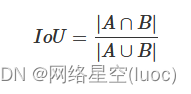
而GIoU公式如下:
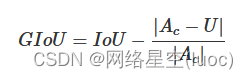
其中Ac
代表两个框最小闭包区域面积,也就是同时包含了预测框和真实框的最小框的面积。
yolov3中提供了IoU、GIoU、DIoU和CIoU等计算方式,以GIoU为例:
if GIoU:  # Generalized IoU https://arxiv.org/pdf/1902.09630.pdf
    c_area = cw * ch + 1e-16  # convex area
    return iou - (c_area - union) / c_area  # GIoU
可以看到代码和GIoU公式是一致的,再来看一下lbox计算部分:
giou = bbox_iou(pbox.t(), tbox[i],
				x1y1x2y2=False, GIoU=True)
lbox += (1.0 - giou).sum() if red == 'sum' else (1.0 - giou).mean()
可以看到box的loss是1-giou的值。
2. lobj部分
lobj代表置信度,即该bounding box中是否含有物体的概率。在yolov3代码中obj loss可以通过arc来指定,有两种模式:
如果采用default模式,使用BCEWithLogitsLoss,将obj loss和cls loss分开计算:
BCEobj = nn.BCEWithLogitsLoss(pos_weight=ft([h['obj_pw']]), reduction=red)
if 'default' in arc:  # separate obj and cls
    lobj += BCEobj(pi[..., 4], tobj)  # obj loss
    # pi[...,4]对应的是该框中含有目标的置信度,和giou计算BCE
    # 相当于将obj loss和cls loss分开计算
如果采用BCE模式,使用的也是BCEWithLogitsLoss, 计算对象是所有的cls loss:
BCE = nn.BCEWithLogitsLoss(reduction=red)
elif 'BCE' in arc:  # unified BCE (80 classes)
    t = torch.zeros_like(pi[..., 5:])  # targets
    if nb:
        t[b, a, gj, gi, tcls[i]] = 1.0 # 对应正样本class置信度设置为1
        lobj += BCE(pi[..., 5:], t)#pi[...,5:]对应的是所有的class
3. lcls部分
如果是单类的情况,cls loss=0
如果是多类的情况,也分两个模式:
如果采用default模式,使用的是BCEWithLogitsLoss计算class loss。
BCEcls = nn.BCEWithLogitsLoss(pos_weight=ft([h['cls_pw']]), reduction=red)
# cls loss 只计算多类之间的loss,单类不进行计算


if 'default' in arc and model.nc > 1:
    t = torch.zeros_like(ps[:, 5:])  # targets
    t[range(nb), tcls[i]] = 1.0 # 设置对应class为1
    lcls += BCEcls(ps[:, 5:], t)  # 使用BCE计算分类loss
如果采用CE模式,使用的是CrossEntropy同时计算obj loss和cls loss。
CE = nn.CrossEntropyLoss(reduction=red)
elif 'CE' in arc:  # unified CE (1 background + 80 classes)
    t = torch.zeros_like(pi[..., 0], dtype=torch.long)  # targets
    if nb:
    t[b, a, gj, gi] = tcls[i] + 1 # 由于cls是从零开始计数的,所以+1
    lcls += CE(pi[..., 4:].view(-1, model.nc + 1), t.view(-1))
    # 这里将obj loss和cls loss一起计算,使用CrossEntropy Loss
以上三部分总结下来就是下图: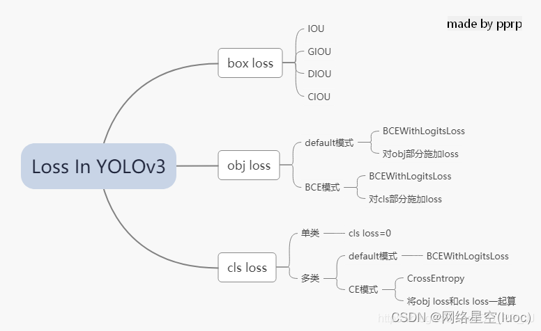
4. 代码
ultralytics版版的yolov3的loss已经和论文中提出的部分大相径庭了,代码中很多地方地方是来自作者的经验。另外,这里读的代码是2020年2月份左右作者发布的版本,关注这个库的人会知道,作者更新速度非常快,在笔者写这篇文章的时候,loss也出现了大幅改动,添加了label smoothing等新的机制,去掉了通过arc来调整loss的机制,简化了loss部分。
这部分的代码添加了大量注释,很多是笔者通过debug得到的结果,理解的时候需要讲一下debug的配置:
- 单类数据集class=1
- batch size=2
- 模型是yolov3.cfg
计算loss这部分代码可以大概上分为两部分,一部分是正负样本选取,一部分是loss计算。
1. 正负样本选取部分
这部分主要工作是在每个yolo层将预设的anchor和ground truth进行匹配,得到正样本,回顾一下上文中在YOLOv3中正负样本选取规则:
- 如果一个预测框与所有的Ground Truth的最大IoU<ignore_thresh时,那这个预测框就是负样本。
- 如果Ground Truth的中心点落在一个区域中,该区域就负责检测该物体。将与该物体有最大IoU的预测框作为正样本(注意这里没有用到ignore thresh,即使该最大IoU<ignore thresh也不会影响该预测框为正样本)
def build_targets(model, targets):
    # targets = [image, class, x, y, w, h]
    # 这里的image是一个数字,代表是当前batch的第几个图片
    # x,y,w,h都进行了归一化,除以了宽或者高

    nt = len(targets)

    tcls, tbox, indices, av = [], [], [], []

    multi_gpu = type(model) in (nn.parallel.DataParallel,
                                nn.parallel.DistributedDataParallel)

    reject, use_all_anchors = True, True
    for i in model.yolo_layers:
        # yolov3.cfg中有三个yolo层,这部分用于获取对应yolo层的grid尺寸和anchor大小
        # ng 代表num of grid (13,13) anchor_vec [[x,y],[x,y]]
        # 注意这里的anchor_vec: 假如现在是yolo第一个层(downsample rate=32)
        # 这一层对应anchor为:[116, 90], [156, 198], [373, 326]
        # anchor_vec实际值为以上除以32的结果:[3.6,2.8],[4.875,6.18],[11.6,10.1]
        # 原图 416x416 对应的anchor为 [116, 90]
        # 下采样32倍后 13x13 对应的anchor为 [3.6,2.8]
        if multi_gpu:
            ng = model.module.module_list[i].ng
            anchor_vec = model.module.module_list[i].anchor_vec
        else:
            ng = model.module_list[i].ng,
            anchor_vec = model.module_list[i].anchor_vec

        # iou of targets-anchors
        # targets中保存的是ground truth
        t, a = targets, []

        gwh = t[:, 4:6] * ng[0]

        if nt:  # 如果存在目标
            # anchor_vec: shape = [3, 2] 代表3个anchor
            # gwh: shape = [2, 2] 代表 2个ground truth
            # iou: shape = [3, 2] 代表 3个anchor与对应的两个ground truth的iou
            iou = wh_iou(anchor_vec, gwh)  # 计算先验框和GT的iou

            if use_all_anchors:
                na = len(anchor_vec)  # number of anchors
                a = torch.arange(na).view(
                    (-1, 1)).repeat([1, nt]).view(-1)  # 构造 3x2 -> view到6
                # a = [0,0,1,1,2,2]
                t = targets.repeat([na, 1])
                # targets: [image, cls, x, y, w, h]
                # 复制3个: shape[2,6] to shape[6,6]
                gwh = gwh.repeat([na, 1])
                # gwh shape:[6,2]
            else:  # use best anchor only
                iou, a = iou.max(0)  # best iou and anchor
                # 取iou最大值是darknet的默认做法,返回的a是下角标

            # reject anchors below iou_thres (OPTIONAL, increases P, lowers R)
            if reject:
                # 在这里将所有阈值小于ignore thresh的去掉
                j = iou.view(-1) > model.hyp['iou_t']
                # iou threshold hyperparameter
                t, a, gwh = t[j], a[j], gwh[j]

        # Indices
        b, c = t[:, :2].long().t()  # target image, class
        # 取的是targets[image, class, x,y,w,h]中 [image, class]

        gxy = t[:, 2:4] * ng[0]  # grid x, y

        gi, gj = gxy.long().t()  # grid x, y indices
        # 注意这里通过long将其转化为整形,代表格子的左上角

        indices.append((b, a, gj, gi))
        # indice结构体保存内容为:
        ''' b: 一个batch中的角标 a: 代表所选中的正样本的anchor的下角标 gj, gi: 代表所选中的grid的左上角坐标 '''
        # Box
        gxy -= gxy.floor()  # xy
        # 现在gxy保存的是偏移量,是需要YOLO进行拟合的对象
        tbox.append(torch.cat((gxy, gwh), 1))  # xywh (grids)
        # 保存对应偏移量和宽高(对应13x13大小的)
        av.append(anchor_vec[a])  # anchor vec
        # av 是anchor vec的缩写,保存的是匹配上的anchor的列表

        # Class
        tcls.append(c)
        # tcls用于保存匹配上的类别列表
        if c.shape[0]:  # if any targets
            assert c.max() < model.nc, 'Model accepts %g classes labeled from 0-%g, however you labelled a class %g. ' \
                                       'See https://github.com/ultralytics/yolov3/wiki/Train-Custom-Data' % (
                                           model.nc, model.nc - 1, c.max())
    return tcls, tbox, indices, av
梳理一下在每个YOLO层的匹配流程:
将ground truth和anchor进行匹配,得到iou
然后有两个方法匹配:
- 使用yolov3原版的匹配机制,仅仅选择iou最大的作为正样本
- 使用ultralytics版版yolov3的默认匹配机制,use_all_anchors=True的时候,选择所有的匹配对
对以上匹配的部分在进行筛选,对应原版yolo中ignore_thresh部分,将以上匹配到的部分中iou<ignore_thresh的部分筛选掉。
最后将匹配得到的内容返回到compute_loss函数中。
2. loss计算部分
这部分就是yolov3中核心loss计算,这部分对照上文的讲解进行理解。
def compute_loss(p, targets, model):
    # p: (bs, anchors, grid, grid, classes + xywh)
    # predictions, targets, model
    ft = torch.cuda.FloatTensor if p[0].is_cuda else torch.Tensor
    lcls, lbox, lobj = ft([0]), ft([0]), ft([0])
    tcls, tbox, indices, anchor_vec = build_targets(model, targets)
    ''' 以yolov3为例,有三个yolo层 tcls: 一个list保存三个tensor,每个tensor中有6(2个gtx3个anchor)个代表类别的数字 tbox: 一个list保存三个tensor,每个tensor形状[6,4],6(2个gtx3个anchor)个bbox indices: 一个list保存三个tuple,每个tuple中保存4个tensor: 分别代表 b: 一个batch中的角标 a: 代表所选中的正样本的anchor的下角标 gj, gi: 代表所选中的grid的左上角坐标 anchor_vec: 一个list保存三个tensor,每个tensor形状[6,2], 6(2个gtx3个anchor)个anchor,注意大小是相对于13x13feature map的anchor大小 '''

    h = model.hyp  # hyperparameters
    arc = model.arc  # # (default, uCE, uBCE) detection architectures
    # 具体使用的损失函数是通过arc参数决定的
    red = 'sum'  # Loss reduction (sum or mean)

    # Define criteria
    BCEcls = nn.BCEWithLogitsLoss(pos_weight=ft([h['cls_pw']]), reduction=red)
    BCEobj = nn.BCEWithLogitsLoss(pos_weight=ft([h['obj_pw']]), reduction=red)
    #BCEWithLogitsLoss = sigmoid + BCELoss
    BCE = nn.BCEWithLogitsLoss(reduction=red)
    CE = nn.CrossEntropyLoss(reduction=red)  # weight=model.class_weights

    # class label smoothing https://arxiv.org/pdf/1902.04103.pdf eqn 3
    # cp, cn = smooth_BCE(eps=0.0)
    # 这是最新的版本中提供了label smoothing的功能,只能用在多类问题

    if 'F' in arc:  # add focal loss
        g = h['fl_gamma']
        BCEcls, BCEobj, BCE, CE = FocalLoss(BCEcls, g), FocalLoss(
            BCEobj, g), FocalLoss(BCE, g), FocalLoss(CE, g)
        # focal loss可以用在cls loss或者obj loss

    # Compute losses
    np, ng = 0, 0  # number grid points, targets
    # np这个命名真的迷,建议改一下和numpy缩写重复
    for i, pi in enumerate(p):  # layer index, layer predictions
        # 在yolov3中,p有三个yolo layer的输出pi
        # 形状为:(bs, anchors, grid, grid, classes + xywh)
        b, a, gj, gi = indices[i]  # image, anchor, gridy, gridx
        tobj = torch.zeros_like(pi[..., 0])
        # tobj = target obj, 形状为(bs, anchors, grid, grid)
        np += tobj.numel() # 返回tobj中元素个数

        # Compute losses
        nb = len(b)
        if nb:
            ng += nb # number of targets 用于最后算平均loss
            # (bs, anchors, grid, grid, classes + xywh)
            ps = pi[b, a, gj, gi] # 即找到了对应目标的classes+xywh,形状为[6(2x3),6]

            # GIoU
            pxy = torch.sigmoid(
                ps[:, 0:2] # 将x,y进行sigmoid
            )  # pxy = pxy * s - (s - 1) / 2, s = 1.5 (scale_xy)
            pwh = torch.exp(ps[:, 2:4]).clamp(max=1E3) * anchor_vec[i]
            # 防止溢出进行clamp操作,乘以13x13feature map对应的anchor
            # 这部分和上文中偏移公式是一致的
            pbox = torch.cat((pxy, pwh), 1)  # predicted box
            # pbox: predicted bbox shape:[6, 4]
            giou = bbox_iou(pbox.t(), tbox[i], x1y1x2y2=False,
                            GIoU=True)  # giou computation
            # 计算giou loss, 形状为6
            lbox += (1.0 - giou).sum() if red == 'sum' else (1.0 - giou).mean()
            # bbox loss直接由giou决定
            tobj[b, a, gj, gi] = giou.detach().type(tobj.dtype)
            # target obj 用giou取代1,代表该点对应置信度

            # cls loss 只计算多类之间的loss,单类不进行计算
            if 'default' in arc and model.nc > 1:
                t = torch.zeros_like(ps[:, 5:])  # targets
                t[range(nb), tcls[i]] = 1.0 # 设置对应class为1
                lcls += BCEcls(ps[:, 5:], t)  # 使用BCE计算分类loss

        if 'default' in arc:  # separate obj and cls
            lobj += BCEobj(pi[..., 4], tobj)  # obj loss
            # pi[...,4]对应的是该框中含有目标的置信度,和giou计算BCE
            # 相当于将obj loss和cls loss分开计算

        elif 'BCE' in arc:  # unified BCE (80 classes)
            t = torch.zeros_like(pi[..., 5:])  # targets
            if nb:
                t[b, a, gj, gi, tcls[i]] = 1.0 # 对应正样本class置信度设置为1
            lobj += BCE(pi[..., 5:], t)
            #pi[...,5:]对应的是所有的class

        elif 'CE' in arc:  # unified CE (1 background + 80 classes)
            t = torch.zeros_like(pi[..., 0], dtype=torch.long)  # targets
            if nb:
                t[b, a, gj, gi] = tcls[i] + 1 # 由于cls是从零开始计数的,所以+1
            lcls += CE(pi[..., 4:].view(-1, model.nc + 1), t.view(-1))
            # 这里将obj loss和cls loss一起计算,使用CrossEntropy Loss
    # 使用对应的权重来平衡,这个参数是作者通过参数搜索(random search)的方法搜索得到的
    lbox *= h['giou']
    lobj *= h['obj']
    lcls *= h['cls']

    if red == 'sum':
        bs = tobj.shape[0]  # batch size
        lobj *= 3 / (6300 * bs) * 2
        # 6300 = (10 ** 2 + 20 ** 2 + 40 ** 2) * 3
        # 输入为320x320的图片,则存在6300个anchor
        # 3代表3个yolo层, 2是一个超参数,通过实验获取
        # 如果不想计算的话,可以修改red='mean'
        if ng:
            lcls *= 3 / ng / model.nc
            lbox *= 3 / ng
    loss = lbox + lobj + lcls
    return loss, torch.cat((lbox, lobj, lcls, loss)).detach()
需要注意的是,三个部分的loss的平衡权重不是按照yolov3原文的设置来做的,是通过超参数进化来搜索得到的,具体请看:【从零开始学习YOLOv3】4. YOLOv3中的参数进化
5. 补充
补充一下BCEWithLogitsLoss的用法,在这之前先看一下BCELoss:
torch.nn.BCELoss的功能是二分类任务是的交叉熵计算函数,可以认为是CrossEntropy的特例。其分类限定为二分类,y的值必须为{0,1},input应该是概率分布的形式。在使用BCELoss前一般会先加一个sigmoid激活层,常用在自编码器中。
计算公式:
![ln=−wn[ynlog(xn)+(1−yn)log(1−xn)]](/img/33/50f21150d0d47b9255ad885dff964d.png)
wn是每个类别的loss权重,用于类别不均衡问题。
torch.nn.BCEWithLogitsLoss的相当于Sigmoid+BCELoss, 即input会经过Sigmoid激活函数,将input变为概率分布的形式。
计算公式:
![ln=−wn[ynlogσ(xn)+(1−yn)log(1−σ(xn))]](/img/55/9c2ea51f2d67de030c185cab20c128.png)
边栏推荐
- Solve the problem of slow access to foreign public static resources
- 分类TAB商品流多目标排序模型的演进
- 【Office】Excel中IF函数的8种用法
- 中非 钻石副石怎么镶嵌,才能既安全又好看?
- Summary of thread and thread synchronization under window
- Prevent browser backward operation
- COMSOL--三维随便画--扫掠
- [crawler] bugs encountered by wasm
- 谜语1
- 项目总结笔记系列 wsTax KT Session2 代码分析
猜你喜欢

How to protect user privacy without password authentication?
COMSOL -- three-dimensional graphics random drawing -- rotation
OneForAll安装使用

The ninth Operation Committee meeting of dragon lizard community was successfully held

中非 钻石副石怎么镶嵌,才能既安全又好看?
How can China Africa diamond accessory stones be inlaid to be safe and beautiful?

13.(地图数据篇)百度坐标(BD09)、国测局坐标(火星坐标,GCJ02)、和WGS84坐标系之间的转换
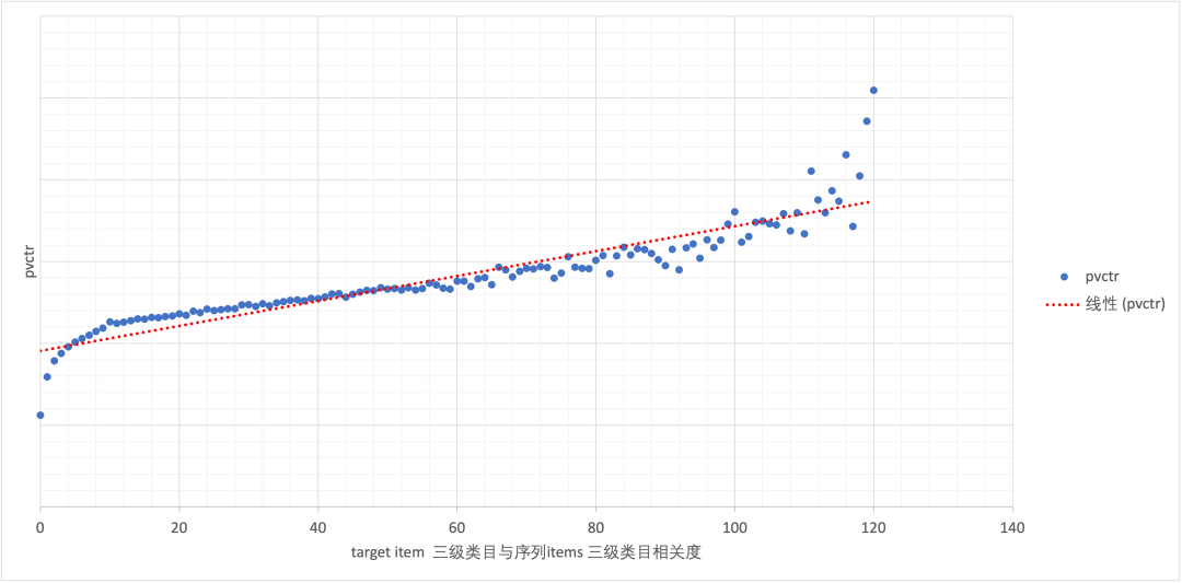
分类TAB商品流多目标排序模型的演进
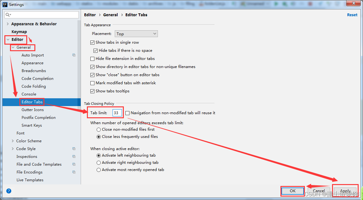
idea设置打开文件窗口个数
7.2 daily study 4
随机推荐
Programmers are involved and maintain industry competitiveness
COMSOL--建立几何模型---二维图形的建立
871. Minimum Number of Refueling Stops
Basics - rest style development
Open3D 欧式聚类
SET XACT_ ABORT ON
居家办公那些事|社区征文
go语言学习笔记-分析第一个程序
阻止瀏覽器後退操作
The ninth Operation Committee meeting of dragon lizard community was successfully held
Mysql统计技巧:ON DUPLICATE KEY UPDATE用法
Harbor image warehouse construction
How does redis implement multiple zones?
Error assembling WAR: webxml attribute is required (or pre-existing WEB-INF/web.xml if executing in
C#实现WinForm DataGridView控件支持叠加数据绑定
SLAM 01. Modeling of human recognition Environment & path
C operation XML file
COMSOL -- establishment of geometric model -- establishment of two-dimensional graphics
Solve the problem of slow access to foreign public static resources
Startup process of uboot: