[point cloud processing paper crazy reading classic version 14] - dynamic graph CNN for learning on point clouds

Abstract

1. background ： For many applications in computer graphics ,point clouds It is a flexible geometric representation , Usually most 3D Raw output of the acquisition device
2. problem ： Even though point clouds Of hand-designed Features have been proposed a long time ago , But recently in image It's very hot convolutional neural networks(CNNs) Indicates that CNN Applied to the point clouds The value of .Point clouds Lack of topology information , So we need to design a model that can recover topology information , So as to enrich point clouds Express the purpose of ability
3. Method ： stay CNN There is an embedded one called EdgeConv Module
   • EdgeConv The module functions in graphs On , Dynamically evaluate each layer of the network graphs Calculate
   • EdgeConv Modules can be exported , And can be embedded in any existing network
   • EdgeConv The module considers local neighborhood information and global shape information
   • EdgeConv It has sort invariance
   • In feature space multi-layer systems affinity Collect the potential long-distance semantic features in the original embedding .
4. Code ：
   • TensorFlow edition
   • PyTorch edition

Method

• In order to mine local geometry , Construct a local neighborhood graph, And apply convolution operation on the edge , Edges connect adjacent pairs of points .
• Article graph Unfixed , Dynamically update at every layer of the network , in other words , One point $kNN$ The elements in the set change from layer to layer in the network , It's through embeddings Sequence calculation .
• Proximity and input in feature space are different , This will lead to the nonlocal diffusion of information in the whole point cloud .

Edge Convolution

remember $\mathbf{X}=\left\{{\mathbf{x}}_1,\dots ,{\mathbf{x}}_n\right\}\subseteq {\mathbb{R}}^F$ Enter a point cloud for , among $n$ Is the number of points ,$F$ It's the dimension of a point , In the simplest case ,$F=3$, Every point includes 3D coordinate ${\mathbf{x}}_i=\left(x_i,y_i,z_i\right)$, In other cases , Colors will also be included 、 Normal vector, etc , At other layers of the network ,$F$ Represents the characteristic dimension of the point .

We calculate a directed graph $\mathcal{G}=(\mathcal{V},\mathcal{E})$ , Represents the local point cloud structure , among $\mathcal{V}=\{1,\dots ,n\}$, $\mathcal{E}\subseteq \mathcal{V}\times \mathcal{V}$ They are vertices and edges . In the simplest case , Construct a $\mathrm{X}$ Of KNN graph $\mathcal{G}$. The graph Include self-loop, Each node points to itself . Define the edge feature as ${\mathbf{e}}_{ij}=h_{\Theta }\left({\mathbf{x}}_i,{\mathbf{x}}_j\right)$, among $h_{\Theta }:{\mathbb{R}}^F\times$${\mathbb{R}}^F\to {\mathbb{R}}^{F^{\prime }}$ It's a nonlinear function , The learnable parameters are $\mathbf{\Theta }$.

Last , By using channel Symmetric aggregation operation in units $\square$ (e.g., $\sum$ or max) Definition EdgeConv operation , Aggregate on edge features associated with all edges emitted from each vertex . In the $i$ Vertex EdgeConv The output is expressed as ：
$${\mathbf{x}}_i^{\prime }=\underset{j:(i,j)\in \mathcal{E}}{\square }{h}_{\Theta }\left({\mathbf{x}}_i,{\mathbf{x}}_j\right)$$
among ${\mathbf{x}}_i$ yes central point,$\left\{{\mathbf{x}}_j:(i,j)\in \mathcal{E}\right\}$ yes ${\mathbf{x}}_i$ Of neigboured points. To make a long story short , Given with $n$ Point $F$ Dimensional point cloud ,EdgeConv Will produce an equal number of points $F^{\prime }$ Dimensional point cloud .

Choice of $h$ and $\square$

$h$ The choice of ：

1. Convolution ：
   $$x_{im}^{\prime }=\sum _{j:(i,j)\in \mathcal{E}}{\mathbf{\theta }}_m\cdot {\mathbf{x}}_j.$$
   among $\Theta =\left({\theta }_1,\dots ,{\theta }_M\right)$ Yes $M$ Different filters Weight coding . Every ${\theta }_m$ All have a relationship with $\mathbf{x}$ The same dimension ,$\cdot$ Represent inner product .
2. PointNet type ：
   $$h_{\Theta }\left({\mathbf{x}}_i,{\mathbf{x}}_j\right)=h_{\Theta }\left({\mathbf{x}}_i\right),$$
   Only encode global shape information , Without considering the local neighborhood structure , Count as EdgeConv A special case of .
3. Atzmon Proposed PCNN type ：
   $$x_{im}^{\prime }=\sum _{j\in \mathcal{V}}\left(h_{\mathbf{\theta }\left({\mathbf{x}}_j\right)}\right)g\left(u\left({\mathbf{x}}_i,{\mathbf{x}}_j\right)\right),$$
   among $g$ It's Gauss kernel,$u$ It is used to calculate the distance in European space .
4. PointNet++ type ：
   $$h_{\mathbf{\Theta }}\left({\mathbf{x}}_i,{\mathbf{x}}_j\right)=h_{\mathbf{\Theta }}\left({\mathbf{x}}_j-{\mathbf{x}}_i\right).$$
   Encode only local information , Divide the whole shape into many blocks , Lost global structure information .
5. The symmetric edge function used in this paper ：
   $$h_{\mathbf{\Theta }}\left({\mathbf{x}}_i,{\mathbf{x}}_j\right)={\bar{h}}_{\mathbf{\Theta }}\left({\mathbf{x}}_i,{\mathbf{x}}_j-{\mathbf{x}}_i\right).$$
   It combines the global shape structure ( By way of ${\mathbf{x}}_i$ Is determined by the coordinates of the center ), Local neighborhood information is also considered ( adopt ${\mathbf{x}}_j-{\mathbf{x}}_i$ obtain ).
   Specially , It can also be expressed by the following formula EdgeConv The operation of ：
   $$e_{ijm}^{\prime }=\mathrm{ReLU}\left({\mathbf{\theta }}_m\cdot \left({\mathbf{x}}_j-{\mathbf{x}}_i\right)+{\mathbf{\varphi }}_m\cdot {\mathbf{x}}_i\right),$$
   And then execute ：
   $$x_{im}^{\prime }=\underset{j:(i,j)\in \mathcal{E}}{\max }{e}_{ijm}^{\prime },$$
   among $\Theta =\left({\theta }_1,\dots ,{\theta }_M,{\varphi }_1,\dots ,{\varphi }_M\right)$.

$\square$ Choose as max

Dynamic Graph Update

Our experiments show that , Use the nearest neighbor in the feature space generated by each layer to recalculate graph It is useful to . This is our method with fixed input graph Working on graph CNN A key difference . This dynamic graph Update is the name of our architecture DGCNN Why .

In each layer , It's different graph ${\mathcal{G}}^{(l)}=\left({\mathcal{V}}^{(l)},{\mathcal{E}}^{(l)}\right)$, Among them the first $l$ The form of the edge of the layer is $\left(i,j_{i1}\right),\dots ,\left(i,j_{i{k}_l}\right)$, That is to say ${\mathbf{x}}_{j_{i1}}^{(l)},\dots ,x_{j_{i{k}_l}}^{(l)}$ It's distance ${\mathbf{x}}_i^{(l)}$ Current $k_l$ A little bit . Our network learns how to construct graph $\mathcal{G}$, It is not fixed before the network starts to predict . At the time of implementation , Calculate the distance matrix in the distance space , Then take the nearest for each single point $k$ A little bit .

Properties

Permutation Invariance

Consider that the output of each layer is ：
$${\mathbf{x}}_i^{\prime }=\underset{j:(i,j)\in \mathcal{E}}{\max }{h}_{\mathbf{\Theta }}\left({\mathbf{x}}_i,{\mathbf{x}}_j\right),$$
because max Is a symmetric function , So the output layer ${\mathrm{x}}_i^{\prime }$ Relative to input ${\mathbf{x}}_j$ It's sort invariant . The global maximum pool operation is also sort invariant for the characteristics of aggregation points .

Translation Invariance

Our operation has a part translation invariance nature , Because the edge function formula is not affected by translation , It can also be selectively affected translation influence . Consider at point ${\mathbf{x}}_j$ Sum point ${\mathbf{x}}_i$ Pan on , When translation $T$ when , Yes ：
$$\begin{array}{rl}{e}_{ijm}^{\prime }& ={\mathbf{\theta }}_m\cdot \left({\mathbf{x}}_j+T-\left({\mathbf{x}}_i+T\right)\right)+{\mathbf{\varphi }}_m\cdot \left({\mathbf{x}}_i+T\right)\\ & ={\mathbf{\theta }}_m\cdot \left({\mathbf{x}}_j-{\mathbf{x}}_i\right)+{\mathbf{\varphi }}_m\cdot \left({\mathbf{x}}_i+T\right)\end{array}$$
If you make ${\mathbf{\varphi }}_m=0$ when , Only consider ${\mathbf{x}}_j-{\mathbf{x}}_i$, Then the operation is completely translational . But the model will lose the acquisition of local information , So it's still part translation invariance.

experiment

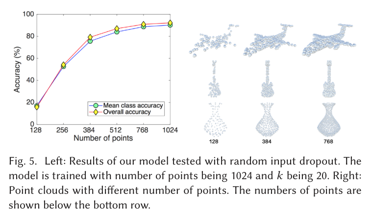
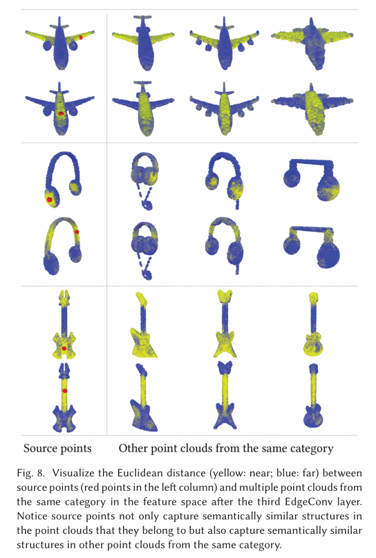
Classification

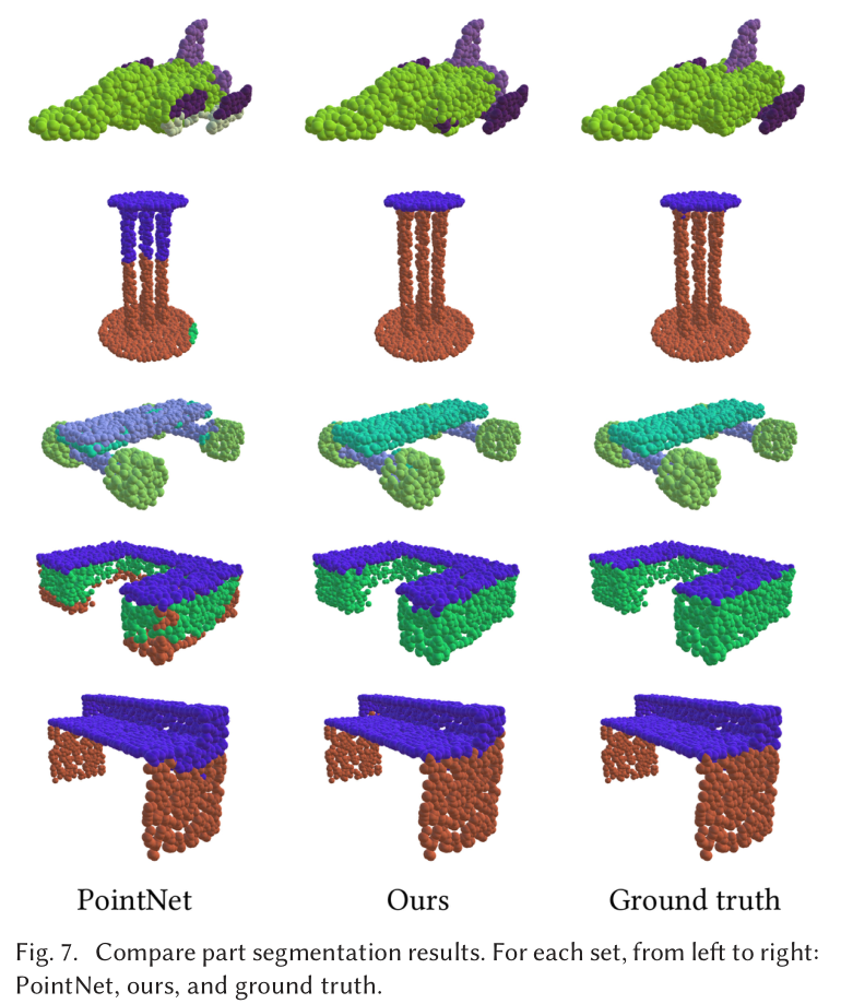
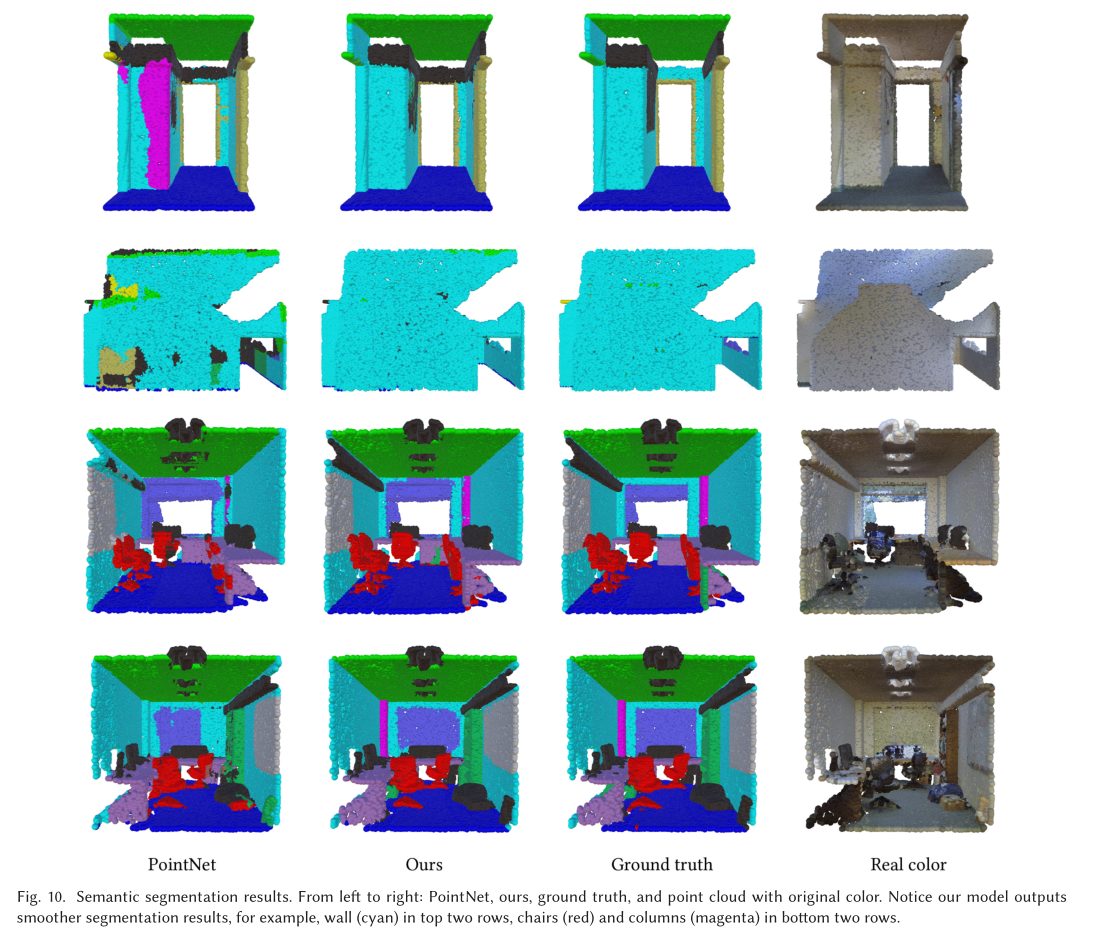
Part Segmentation

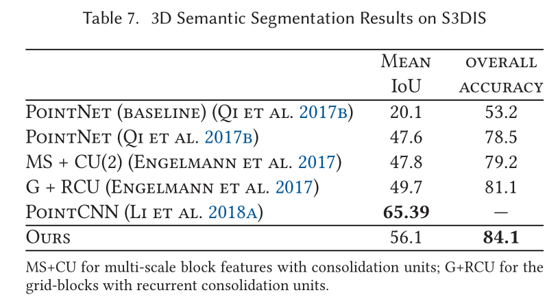
Indoor Scene Segmentation

expectation

1. Improve the speed of the model by combining faster data formats , Use multivariate groups instead , Don't look for the relationship between point pairs
2. Design a non shared transformer The Internet , At every local patch They are all different , More flexibility

New words

1. dub v go by the name of …
2. arguably adv Can be said to be
3. emanate v issue