当前位置:网站首页>Federated reconnaissance: efficient, distributed, class incremental learning paper reading + code analysis
Federated reconnaissance: efficient, distributed, class incremental learning paper reading + code analysis
2022-06-12 07:18:00 【Programmer long】
The address of the paper is here
One . Introduce
In the paper , The author puts forward the concept of joint reconnaissance , This is a new kind of learning problem , The distributed model should be able to learn new concepts independently , And effectively share this knowledge . Usually in joint learning , A single static class set is learned by each client . contrary , Federal reconnaissance requires that each client can learn a growing set of classes , And effectively communicate previously observed and new class knowledge with other clients . This kind of communication about learning can obtain knowledge from customers ; It is then expected that the final merged model supports a superset of the classes exposed by each client . The merged model can then be deployed back to the client for further learning .
1.1 Early work
Continuous learning : Continuous learning of new concepts is an open and long-term problem. There is no apparent unified solution in machine learning and artificial intelligence . Although deep neural networks have been proved to be very effective in a wide range of tasks , But there are ways to continuously integrate new information , At the same time, remembering previously learned concepts can become inefficient . In this work , Let's suppose we access a set of pre training data , And explore algorithms , Allows efficient and accurate learning of the order of new classes .
Federal learning : Unlike continuous learning , Under the guidance of the central server , Iteratively train a common model for data on decentralized devices ( At present, there are also personalized based to adapt to various customers ). I wrote an article before Blog , This paper introduces the federal continuous learning model , Similar to the background of this article . However, this article focuses on the direct sharing of class knowledge
1.2 contribution
An effective federal investigation system must solve the efficient learning of new classes and the preservation and transfer of knowledge . therefore , The author takes the ordinary random gradient descent as the lower bound ,iCaRL The algorithm is used for the comparison of federal investigation and the joint distribution of all training data of all customers SGD As the upper bound .
hypothesis , When a pre trained data set is available , The prototype network is a powerful baseline ( After the prototype network, I will write another blog ), The reason is :
It can compress concepts into relatively small carriers , The so-called prototype , So as to realize efficient communication
In Africa iid When learning from data , Robustness to catastrophic forgetting
During model merging , There is no need for gradient based learning or hyperparametric tuning , So as to realize rapid knowledge transfer .
The author puts forward Federated prototypical network framework , Learn about class increments .
Two . Federal investigation statement
2.1 System requirements
Federal reconnaissance requires continuous learning for each client device 、 Efficient communication and knowledge consolidation . Inspired by applications that learn new classes on a large number of distributed client devices , We define the following requirements of the federal reconnaissance learning system :
- Each client model should be able to learn new classes in place from several examples , And it can improve the accuracy as more examples appear .
- After learning the new class , Every model should not forget the classes you've seen before . in other words , Models should not suffer catastrophic forgetting .
- In order to reduce communication costs , And realize distributed learning under the condition of limited bandwidth , The federal reconnaissance system should be able to compress information before transmission .
- Last , In order to avoid expensive retraining of all data on the central server every time a customer opportunities to a new class , The federated reconnaissance system should be able to quickly incorporate the knowledge of new classes learned by the distributed client model .
The specific requirements for the actual implementation of federal reconnaissance will certainly determine the details and relative importance of each requirement .
2.2 Problem definition
Federal investigation consists of a set of clients C : = { c i ∣ i ∈ 1... C } \mathbb{C}:=\{c_i|i\in 1...C\} C:={ ci∣i∈1...C}, Every client is experiencing an increasing number of classes M i , t : = { p ( y = j ∣ x ) ∣ j ∈ 1... M j } \mathbb{M}_{i,t}:=\{p(y=j|x)|j\in 1...M_j\} Mi,t:={ p(y=j∣x)∣j∈1...Mj}. among C C C Represents the total number of clients , M i M_i Mi Represents the total number of classes that can be distinguished by a client , A class consists of probability p ( y = j ∣ x ) p(y=j|x) p(y=j∣x) Through the label j and x To said . The job of the central server is to merge the client's knowledge of classes M t = ⋃ i = 1 C M i , t \mathbb{M}_t=\bigcup^C_{i=1}\mathbb{M}_{i,t} Mt=⋃i=1CMi,t The updated model is then deployed and the model M t \mathbb{M}_t Mt Return to C \mathbb{C} C. One client C i C_i Ci You can train by directly using a set of labeled examples to reach a new class { ( x , y ) ∣ ( x , y ) ∈ X j × Y j } \{(x,y)|(x,y)\in X_j \times Y_j\} { (x,y)∣(x,y)∈Xj×Yj}, Or exchange compressed knowledge , Make the client approximate estimation p ( y = j ∣ x ) p(y=j|x) p(y=j∣x).
An effective federal investigation system needs to effectively evaluate our predictions p ( y ^ = j ∣ x ) p(\hat{y}=j|x) p(y^=j∣x) Whether it is a direct learning sample or not j Or get knowledge from other clients . Therefore, the distributed objective function of our federal investigation learning system at any time is the average loss of the client :
L = 1 C ∑ i = 1 C 1 J i ∑ j = 1 J i 1 K i , j ∑ k = 1 K i , j H ( y ^ i , j , k , y i , j , k ) (1) \mathcal{L}=\frac{1}{\mathbb{C}}\sum^{\mathbb{C}}_{i=1}\frac{1}{J_i}\sum^{J_i}_{j=1}\frac{1}{K_{i,j}}\sum^{K_{i,j}}_{k=1}H(\hat{y}_{i,j,k},y_{i,j,k}) \tag 1 L=C1i=1∑CJi1j=1∑JiKi,j1k=1∑Ki,jH(y^i,j,k,yi,j,k)(1)
among J i J_i Ji Represents a client i The total number of all classes that have been encountered , K i , j K_{i,j} Ki,j Represents a client i Upper part j Number of examples of classes ,H Calculate our predicted and real values for cross entropy loss . For the sake of simple calculation , Assume that the number of clients is fixed throughout the deployment process , Although it's easy to scale to a variable number of clients over time .
At every moment t, A dataset with few examples D t D_t Dt Born with the environment . Federal investigation faces two problems : The client learns from scratch p ( X , Y ) p(X,Y) p(X,Y) And base classes B \mathbb{B} B A subset of is used for pre training . aggregate B \mathbb{B} B Similar to the meta training set in meta learning , We hope that customers will learn more and more superset classes, including those after pre training in basic classes and domain classes B \mathbb{B} B. In practice , Access representation B \mathbb{B} B The data set is a reasonable assumption , Because before the federal investigation system is deployed , You can usually measure the number of pre training classes .
After model merging , We define the expected loss by getting the expectation of the class :
L t = 1 ∣ M t ∣ ∑ j = 1 ∣ M t ∣ 1 K i , j ∑ k = 1 K i , j H ( y ^ i , j , k , y i , j , k ) (2) \mathcal{L}_t=\frac{1}{|\mathbb{M}_t|}\sum^{|\mathbb{M}_t|}_{j=1}\frac{1}{K_{i,j}}\sum^{K_{i,j}}_{k=1}H(\hat{y}_{i,j,k},y_{i,j,k}) \tag 2 Lt=∣Mt∣1j=1∑∣Mt∣Ki,j1k=1∑Ki,jH(y^i,j,k,yi,j,k)(2)
Accuracy rate is :
L t = 1 ∣ M t ∣ ∑ j = 1 ∣ M t ∣ 1 K i , j ∑ k = 1 K i , j [ y ^ i , j , k = y i , j , k ] (3) \mathcal{L}_t=\frac{1}{|\mathbb{M}_t|}\sum^{|\mathbb{M}_t|}_{j=1}\frac{1}{K_{i,j}}\sum^{K_{i,j}}_{k=1}[\hat{y}_{i,j,k}=y_{i,j,k}] \tag 3 Lt=∣Mt∣1j=1∑∣Mt∣Ki,j1k=1∑Ki,j[y^i,j,k=yi,j,k](3)
At every moment t, Each client model first presents some tagged new class data , Then evaluate the super of this new class and the data of all classes in its history . After local training , The client sends the information to the server , Choose to communicate new class information or update the information of the class you saw before , The server combines the information of multiple clients . After this model is evaluated , We evaluate the accuracy of set and domain classes . The process of learning and exchanging knowledge by the client is repeated in the server . therefore , We need to minimize the equation (1) On mission { t ∈ N ∣ t ≤ T } \{t \in \mathbb{N}|t\le T\} { t∈N∣t≤T}:
min t ∈ 1 , . . . T E [ L t ] (4) \min_{t\in 1,...T}\mathbb{E}[\mathcal{L_t}] \tag 4 t∈1,...TminE[Lt](4)
perhaps , After learning a fixed number of tasks :
min L t = T (5) \min \mathcal{L}_{t=T} \tag{5} minLt=T(5)
For simplicity , Highlight the challenges of distributed learning , According to (5) To assess the .
3、 ... and . Method
3.1 The algorithm of learning
( Here the author says what methods he has compared , Because this blog is mainly about learning ideas , So don't write )
3.2 Federal prototype network (Federated Prototypical Networks)
We propose to use prototype network to effectively learn new classes in sequence . Because the prototype network is not based on gradient , So when learning new classes , Through discriminative pre training for enough classes , It can make them robust to catastrophic forgetting . When evaluating on a federal reconnaissance benchmark , We can simply store the previous prototype ( variance ) And the number of examples used to calculate the previous prototype to calculate the average value of each class ( If necessary , And variance ) Unbiased estimation of . We defined the prototype network according to :
z = f θ ( x i ) (6) z = f_\theta(x_i) \tag 6 z=fθ(xi)(6)
z ˉ j = 1 ∣ S j ∣ ∑ ( x i , y i ) ∈ S j f θ ( x i ) (7) \bar{z}_j=\frac{1}{|S_j|}\sum_{(x_i,y_i)\in S_j}f_\theta(x_i) \tag 7 zˉj=∣Sj∣1(xi,yi)∈Sj∑fθ(xi)(7)
among f f f For a person who θ \theta θ and S j S_j Sj Parameterized neural embedding network ( S j S_j Sj Expressed as a support set ). A prototype network is trained to minimize cross entropy loss on query examples , The prediction class is regarded as the negative Euclidean distance between query embedding and supporting data prototypes softmax:
p θ ( y = j ∣ x ) = e x p ( − d ( f θ ( x ) , z ˉ j ) ) ∑ j ′ ∈ J e x p ( − d ( f θ ( x ) , z ˉ j ′ ) ) (8) p_\theta(y=j|x)=\frac{exp(-d(f_\theta(x),\bar{z}_j))}{\sum_{j'\in J}exp(-d(f_\theta(x),\bar{z}_{j'}))} \tag 8 pθ(y=j∣x)=∑j′∈Jexp(−d(fθ(x),zˉj′))exp(−d(fθ(x),zˉj))(8)
Now? , We hope to be able to calculate unbiased estimates for prototypes of classes observed by multiple clients in the current time step or in previous history . In order to improve the efficiency of storage and communication , We can store the previous prototype and the number of examples used to calculate it , To calculate an unbiased running average for each prototype , Instead of storing all the original examples of a class or even all the embedded examples :
μ t = k t − 1 μ t − 1 k t + ( k t − k t − 1 ) z ˉ j k t (9) \mu_t = \frac{k_{t-1}\mu_{t-1}}{k_t}+\frac{(k_t-k_{t-1})\bar{z}_j}{k_t} \tag 9 μt=ktkt−1μt−1+kt(kt−kt−1)zˉj(9)
among k t k_t kt It's in time t Classes observed on j The number of , μ t \mu_t μt For the class j Of all the examples above z z z Average value . Finally, according to uncle's Theorem , We can work out μ ∗ \mu^* μ∗:
z ˉ k → a . s . μ ∗ a s k → ∞ (10) \bar z_k \xrightarrow{a.s.} \mu^*\ \ \ \ as\ k\rightarrow \infty \tag {10} zˉka.s.μ∗ as k→∞(10)
In practical terms , The relevant values cannot be ignored , Therefore, a more stable method is used to calculate :
μ t ← μ t − 1 + k t − k t − 1 k t ( z ˉ − μ t − 1 ) (11) \mu_t \leftarrow \mu_{t-1}+\frac{k_t-k_{t-1}}{k_t}(\bar z - \mu_{t-1}) \tag{11} μt←μt−1+ktkt−kt−1(zˉ−μt−1)(11)
The specific algorithm is shown in the figure below :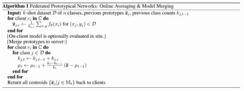
Four . Key code interpretation
Code address point here
in general , This paper is based on prototypical network To carry out , If the prototypical network If you have questions, you can also look at the code , Simple code .
4.1 Meta training part
The first is that we need to define prototypical The Internet , That is to calculate z Come on .
class PrototypicalNetwork(nn.Module):
    def __init__(
        self,
        in_channels,
        out_channels,
        hidden_size=64,
        pooling: Optional[str] = None,
        backbone: str = "4conv",
        l2_normalize_embeddings: bool = False,
        drop_rate: Optional[float] = None,
    ):
        """Standard prototypical network"""
        super().__init__()
        self.supported_backbones = {
    "4conv", "resnet18"}
        assert backbone in self.supported_backbones
        self.pooling = pooling
        self.backbone = backbone
        self.in_channels = in_channels
        self.out_channels = out_channels
        self.hidden_size = hidden_size

		##  The network layer , It's used here 4conv That is to say 4 A winder layer
        if self.backbone == "resnet18":
            self.encoder = build_resnet18_encoder(drop_rate=drop_rate)
        elif self.backbone == "4conv":
            self.encoder = build_4conv_protonet_encoder(
                in_channels, hidden_size, out_channels, drop_rate=drop_rate
            )
        else:
            raise ValueError(
                f"Unsupported backbone {
      self.backbone} not in {
      self.supported_backbones}"
            )

        if self.pooling is not None:
            assert self.pooling in SUPPORTED_POOLING_LAYERS
        if self.pooling == "Gem":
            self.gem_pooling = GeM()
        else:
            self.gem_pooling = None

        self.l2_normalize_embeddings = l2_normalize_embeddings

    def forward(self, inputs):
        batch, nk, _, _, _ = inputs.shape
        inputs_reshaped = inputs.view(
            -1, *inputs.shape[2:]
        )  # -> [b * k * n, input_ch, rows, cols]

        embeddings = self.encoder(
            inputs_reshaped
        )  # -> [b * n * k, embedding_ch, rows, cols]
        # TODO: add optional support for half for further prototype/embedding compression
        # embeddings = embeddings.type(torch.float16)
        # RuntimeError: "clamp_min_cpu" not implemented for 'Half'
        if self.pooling is None:
            embeddings_reshaped = embeddings.view(
                *inputs.shape[:2], -1
            )  # -> [b, n * k, embedding_ch * rows * cols] (4608 for resnet 18)
        elif self.pooling == "average":
            embeddings_reshaped = embeddings.mean(dim=[-1, -2]).reshape(
                batch, nk, -1
            )  # -> [b, n * k, embedding_ch] (512 for resnet 18)
        elif self.pooling == "Gem":
            embeddings_reshaped = (
                self.gem_pooling(embeddings).squeeze(-1).squeeze(-1).unsqueeze(0)
            )
        else:
            raise ValueError
        if self.l2_normalize_embeddings:
            embeddings_reshaped = torch.nn.functional.normalize(
                embeddings_reshaped, p=2, dim=2
            )
        return embeddings_reshaped
It's complicated , In fact, that is 4 Composed of three convolutions , The author here hidden_size by 64(64 individual 3*3 Convolution kernel ), So if you say batch Of x by [1,25,1,28,28]( Similar to meta learning , first 1 Indicates that there is a task ,25 Indicates the amount of data contained in a task , Here is 5way5shot So it is 25, Third 1 Means the passage , Then the picture ), after encorder And then it became :[25,64,1,1], Then it changed its shape to encorder = [1,25,64] Calculate after convenience .
Let's look at the calculation z:
z ˉ j = 1 ∣ S j ∣ ∑ ( x i , y i ) ∈ S j f θ ( x i ) \bar{z}_j=\frac{1}{|S_j|}\sum_{(x_i,y_i)\in S_j}f_\theta(x_i) zˉj=∣Sj∣1(xi,yi)∈Sj∑fθ(xi)
That is, average the samples of a class , The code is as follows :
def get_prototypes(
    embeddings,
    n_classes,
    k_shots_per_class,
    return_sd: bool = False,
    prototype_normal_std_noise: Optional[float] = None,
):
    batch_size, embedding_size = embeddings.size(0), embeddings.size(-1)
    embeddings_reshaped = embeddings.reshape(
        [batch_size, n_classes, k_shots_per_class, embedding_size]
    )
    prototypes = embeddings_reshaped.mean(2)
    # print(f"Prototype shape for {n_classes} [batch, n_classes, embedding_size]: {prototypes.shape}")
    assert len(prototypes.shape) == 3

    if prototype_normal_std_noise is not None:
        prototypes += torch.normal(
            torch.zeros_like(prototypes),
            torch.ones_like(prototypes) * prototype_normal_std_noise,
        )
    if return_sd:

        return prototypes, embeddings_reshaped.std(2)
    return prototypes
First of all, to our 5way5shot Split encorder, Turn into [1,5,5,64], Then average the samples in each of our classes ( That is to say 5 individual example Average ), Calculate the z for :[1,5,64]
Then the last thing is to calculate loss:
p θ ( y = j ∣ x ) = e x p ( − d ( f θ ( x ) , z ˉ j ) ) ∑ j ′ ∈ J e x p ( − d ( f θ ( x ) , z ˉ j ′ ) ) p_\theta(y=j|x)=\frac{exp(-d(f_\theta(x),\bar{z}_j))}{\sum_{j'\in J}exp(-d(f_\theta(x),\bar{z}_{j'}))} pθ(y=j∣x)=∑j′∈Jexp(−d(fθ(x),zˉj′))exp(−d(fθ(x),zˉj))
To our query set It's also going on encorder And then with our z Calculation softmax, The corresponding code is as follows :
def prototypical_loss(
    prototypes, embeddings, targets, sum_loss_over_examples, **kwargs
):
	##  Ask for distance d
    squared_distances = torch.sum(
        (prototypes.unsqueeze(2) - embeddings.unsqueeze(1)) ** 2, dim=-1
    )
    if sum_loss_over_examples:
        reduction = "sum"
    else:
        reduction = "mean"
     ## \frac{exp(-d(f_\theta(x),\bar{z}_j))}{\sum_{j'\in J}exp(-d(f_\theta(x),\bar{z}_{j'}))}
    return F.cross_entropy(-squared_distances, targets, reduction=reduction, **kwargs)
Keep iterating and updating our encorder The parameters in the layer can .
4.2 Meta test part —— Class increment
After training , our enocrder Achieve the best parameters θ ∗ \theta^* θ∗, Now let's do the meta test , Test the class increment .
First, the network layer is the same as meta training , Just load our parameters directly . Because it is class increment , We need to add one class by one . Empathy , Split the data of a class into train set and test set, here train Each class in contains 15 Samples ,test Then for 5 individual . It is assumed that n Classes , First of all, from the train set( Only the current class is calculated ) Calculation encorder from [1,15,1,28,28] Turn into [1,15,64], Calculated after prototype Turn into [1,64], Plus the first few classes stored before prototype Turn into :[1,n,64].test set Also through encorder Turn into [1,5*n,64].
train_embeddings = self.forward(train_inputs)
test_embeddings = self.forward(test_inputs)
##  Calculation z
all_class_prototypes = self._get_prototypes(
    train_embeddings, train_labels, n_train_classes, k_shots
)
Calculation z, Because only the information of the current class , Therefore, we need to store the previous class z, Then together concat that will do .
def _get_prototypes(
    self,
    train_embeddings: torch.Tensor,
    train_labels: torch.Tensor,
    n_train_classes: int,
    k_shots: int,
):
    new_prototypes = get_prototypes(
        train_embeddings, n_train_classes, k_shots
    )  # -> [b, n, features]

    # Add each prototype to the model:
    assert len(new_prototypes.shape) == 3
    assert new_prototypes.shape[0] == 1
    new_prototypes = new_prototypes[
        0
    ]  # Assume single element in batch dimension. Now [n_train_classes, features]
    class_indices = train_labels.unique()
    for i, cls_index in enumerate(class_indices):
        self.update_prototype_for_class(
            cls_index, new_prototypes[i, :], train_labels.shape[1]
        )
    all_class_prototypes = [
        self.prototypes[key] for key in sorted(self.prototypes.keys())
    ]
    all_class_prototypes: torch.FloatTensor = torch.stack(
        all_class_prototypes, dim=0
    ).unsqueeze(
        0
    )  # -> [1, n, features]
    return all_class_prototypes
Then calculate the distance , Then calculate the subscript with the smallest distance between the two is the prediction .
def get_protonet_accuracy(
    prototypes: torch.FloatTensor,
    embeddings: torch.FloatTensor,
    targets: Union[torch.Tensor, torch.LongTensor],
    jsd: bool = False,
    mahala: bool = False,
) -> torch.FloatTensor:
    sq_distances = torch.sum(
        (prototypes.unsqueeze(1) - embeddings.unsqueeze(2)) ** 2, dim=-1
    )
_, predictions = torch.min(sq_distances, dim=-1)
return get_accuracy(predictions, targets)
边栏推荐
- Pyhon的第四天
- Study on display principle of seven segment digital tube
- Keil installation of C language development tool for 51 single chip microcomputer
- 8 IO Library
- SQL Server 2019 installation error. How to solve it
- "I was laid off by a big factory"
- Pyhon的第六天
- Federated meta learning with fast convergence and effective communication
- Why must coordinate transformations consist of publishers / subscribers of coordinate transformation information?
- Database syntax related problems, solve a correct syntax
猜你喜欢

C language sizeof strlen
Detailed explanation of 14 registers in 8086CPU

Kotlin插件 kotlin-android-extensions

2022年G3锅炉水处理复训题库及答案

2022电工(初级)考试题库及模拟考试

Pyhon的第四天
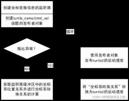
Detailed explanation of coordinate tracking of TF2 operation in ROS (example + code)
![‘CMRESHandler‘ object has no attribute ‘_timer‘,socket.gaierror: [Errno 8] nodename nor servname pro](/img/de/6756c1b8d9b792118bebb2d6c1e54c.png)
‘CMRESHandler‘ object has no attribute ‘_timer‘,socket.gaierror: [Errno 8] nodename nor servname pro

2022年危险化学品经营单位安全管理人员特种作业证考试题库及答案

AI狂想|来这场大会,一起盘盘 AI 的新工具!
随机推荐
Paddepaddl 28 supports the implementation of GHM loss, a gradient balancing mechanism for arbitrary dimensional data (supports ignore\u index, class\u weight, back propagation training, and multi clas
Win10 list documents
d中的解耦
Dynamic coordinate transformation in ROS (dynamic parameter adjustment + dynamic coordinate transformation)
Learning to continuously learn paper notes + code interpretation
How to update kubernetes certificates
i. Mx6ul porting openwrt
Pyhon的第五天
Thoroughly understand the "rotation matrix / Euler angle / quaternion" and let you experience the beauty of three-dimensional rotation
Android studio uses database to realize login and registration interface function
D cannot use a non CTFE pointer
1. Foundation of MySQL database (1- installation and basic operation)
Keil installation of C language development tool for 51 single chip microcomputer
Tradeoff and selection of SWC compatible Polyfill
postman拼接替换参数循环调用接口
私有协议的解密游戏:从秘文到明文
RT thread studio learning (x) mpu9250
Detailed explanation of memory addressing in 8086 real address mode
循环链表和双向链表—课上课后练
新知识:Monkey 改进版之 App Crawler