当前位置：网站首页>LightGBM原理及天文数据中的应用

LightGBM原理及天文数据中的应用

2022-07-02 21:33:00 【yellow】

1 LightGBM 简介

Light gradient boosting machine(LightGBM)是一个带有单边梯度采样(gradient-based one-side sampling，GOSS)与互斥特征捆绑(exclusive feature bundling，EFB)的梯度提升决策树(gradient boosting decision tree，GBDT)。
LightGBM使用直方图方法(histogram-based algorithm)寻找每棵树的最佳分裂节点，因此速度比传统GBDT更快。
LightGBM使用GOSS排除每棵树中残差小的样本，并关注大残差样本(减少样本量，提升模型泛化能力)；LightGBM使用EFB关注特征维度比较大的样本，减少稀疏特征的影响(类似于PCA降维)。

2 LightGBM原理

LightGBM是一个带有单边梯度采样与互斥特征捆绑的梯度提升决策树模型，每一棵决策树使用直方图方法寻找最佳分裂节点。

以下叙述仅考虑大样本回归预测，且不针对互斥特征捆绑进行叙述(因为特征工程往往比互斥特征捆绑更优秀，使用LightGBM对特征处理时，尽量使用其他方法吧；另一方面笔者所用天文测光数据特征维度仅为6，互斥特征捆绑起不到作用，等后期使用光谱数据时，再来研究补充互斥特征捆绑的原理)！

2.1 梯度提升决策树(GBDT)

在机器学习领域，若一模型的性能略优于随机猜测，则可将该模型称为弱学习器。GBDT是采用回归决策树作为弱学习器的一类Boosting集成模型，即以串联方式构建多个回归决策树，最终回归预测为各决策树之和(也可以加权求和)。本节详细介绍GBDT原理，部分内容参考Friedman(2001)。

假如为个样本集，其中为第个样本的个特征维度，为的响应值。输入，GBDT输出值为：

其中为GBDT中回归决策树的数量，是第个回归决策树，为第个回归决策树关于第的预测值。GBDT采用下述4步来计算：

1.初始化。
2.计算残差值 ,得到样本集：

3.拟合样本集O得到回归决策树。
4.更新。

集成模型往往在上述第3步采用不同的方式拟合。GBDT采用最简单的方式进行拟合决策树，即，样本集O被父节点递归性分为两个区域（左、右孩子节点）。每个区域（左、右孩子节点）的输出值通过执行以下3步构建二叉决策树确定：

1.从根节点开始，选择最佳分割变量和最优分割点（变量的取值），并最小化两个区域的预测值和实际值（左、右子节点）的均方误差：

其中

且分别为左、右节点的预测值。

2.在第1步之后，使用左、右子节点作为下一次拆分的新父节点。按照第1步，拆分新的父节点。
3.重复第1步与第2步建立建立完成！

经过上述3步后，建立完成！然而，集合中的残差大小不同，小残差意味着GBDT预测值几乎收敛于真实值，再次拟合小残差样本将增加模型过拟合风险，且增加构建耗时。为了克服这些问题，单边梯度采样与直方图方法加入到了GBDT，这也是LightGBM模型的优点。

2.2 单边梯度采样(GOSS)

单边梯度采样是一种区别对待数据集中不同残差的统计学方法。该方法通过随机剔除数据集中小残差样本，即改变GBDT第2步中样本量提升模型的泛化能力。单边梯度采样通过下述3步实现：

1.将数据集中的残差进行排序，不妨设：

2.将第一步前残差对应数据集记为集合；剩余残差对应数据集记为集合，包含小残差。

其中。

3.从集合中随机取记为集合。集合只包含部分小残差样本，为了减少数据分布对模型的影响，对集合中残差乘以系数，即，

其中。

上述3步对应着GBDT第2步计算残差构造集合，Ke et al.(2017)证明了相比于GBDT模型，单边梯度采样通过关注大样本残差提升了模型泛化能力。

2.2 直方图方法(Histogram-based Algorithm)

回归决策树寻找最佳分裂节点是一个耗时的过程，这也是GBDT速度慢的主要原因。为了缓解该问题，Ke et al.(2017)使用直方图方法将连续变量值存储到离散箱子中，并使用这些箱子在训练期间构建特征直方图。即，第个变量升序排列后划分到个箱子中，每个箱子包含个样本。

此时，寻找第个变量的最佳分裂节点从范围变为了。最终，在集合中，类似于公式(1)，通过下述公式得到最佳分裂节点，进而构造出最佳回归决策树。

其中

且分别为左、右节点的预测值。

直方图方法通过减少GBDT的第3步中分裂节点的数量(从降低到个，其中远大于 )达到加速的效果。

3 LightGBM的应用

3.1 相关环境与依赖包

虚拟环境：Python 3.6.2
相关包：LightGBM 3.2.1 + bayesian-optimization 1.2.0 + pandas 1.1.5 + numpy 1.19.5 + matplotlib 3.3.3 + scikit-learn 0.24.2
相关包下载方式采用 pip(或者conda) + install + 包名称(注意版本号)，如 pip install lightgbm==3.2.1。

3.2 数据集介绍

实验目的：使用巡天测光数据(星等)预测恒星大气物理参数。
输入变量：X，来源于SAGE巡天与Pan-STARRS DR1交叉得到的测光数据(uvgriz，6个变量)。
输出变量：y，来源于APOGEE DR16恒星大气物理参数(有效温度，log g表面重力加速度，[Fe/H]金属丰度)。
数据集划分说明：37979样本量，按8：2划分训练集与测试集，在训练集中使用贝叶斯优化进行交叉验证调参。

3.3 Python代码实现(以为例，log g与[Fe/H]类似)

调库

# 1. 数据分析常规库
import pandas as pd
import numpy as np
import matplotlib.pyplot as plt
import matplotlib

# 2. 数据集划分库
from sklearn.model_selection import train_test_split, cross_val_score

# 3. 数据处理、特征构造库
from sklearn.preprocessing import MinMaxScaler
from sklearn.decomposition import PCA

# 4. 评价指标库
import sklearn.metrics as sm

# 5. 模型调参贝叶斯优化库
from bayes_opt import BayesianOptimization

# 6. 调用LightGBM库
import lightgbm as lgb

# 7. 可视化决策树库，需要提前下载Graphviz，否则注释掉即可！
import os
os.environ["PATH"] += os.pathsep + 'D:/Graphviz/bin'

# 8. 画图设置微调
matplotlib.rcParams["font.family"] = "SimHei"
matplotlib.rcParams["axes.unicode_minus"] = False
# 将x、y轴的刻度线方向设置向内
plt.rcParams['xtick.direction'] = 'in'
plt.rcParams['ytick.direction'] = 'in'

数据读取与特征构造

# 9. 数据集读取，重命名列名称。
data = pd.read_csv("new_data.csv")
x_data = data[["UMAG", "VMAG", "RMAG", "IMAG", "ZMAG", "GMAG"]]
y_data = data["TEFF"]
x_data.columns = ["u", "v", "r", "i", "z", "g"]
y_data.columns = ["Teff"]

# 10. 数据集划分，设置随机种子使得模型可复现。
x_train, x_test, y_train, y_test = train_test_split(x_data, y_data, train_size=0.8, random_state=1)

# 11. 归一化自变量X，测试集按照训练集方式进行归一化。
scaler1 = MinMaxScaler().fit(x_train)
x_train = scaler1.transform(x_train)
x_test = scaler1.transform(x_test)

# 12. 主成分变换自变量X，测试集按照训练集方式进行，并重命名列名称。
pca = PCA(n_components=6, random_state=666).fit(x_train)
x_train = pca.transform(x_train)
x_test = pca.transform(x_test)
x_train = pd.DataFrame(x_train, columns=["F1", "F2", "F3", "F4", "F5", "F6"])
x_test = pd.DataFrame(x_test, columns=["F1", "F2", "F3", "F4", "F5", "F6"])

贝叶斯优化调参

# 13. 贝叶斯优化目标函数的设计：LGBM_cv()。函数中变量为LightGBM模型待调整参数，使用5折交叉验证进行贝叶斯调参！
# top_rate, other_rate分别为LIghtGBM模型中的a与b，即大残差与小残差样本比例。
# 直方图方法主要是加速，此处不作为超参数调整，因为我们重视LightGBM的速度，因此取默认值255。
def LGBM_cv(learning_rate, num_leaves, max_depth, subsample, min_child_samples, n_estimators, feature_fraction, feature_fraction_bynode, lambda_l2, top_rate, other_rate
          ):
    val = cross_val_score(lgb.LGBMRegressor(objective='regression_l2',
                            boosting_type="goss",
                            top_rate=top_rate,
                            other_rate=other_rate,
                            random_state=666,
                            learning_rate=learning_rate,
                            num_leaves=int(num_leaves),
                            max_depth=int(max_depth),
                            subsample=subsample,
                            min_child_samples=int(min_child_samples),
                            n_estimators=int(n_estimators),
                            colsample_bytree=feature_fraction,
                            feature_fraction_bynode=feature_fraction_bynode,
                            reg_lambda=lambda_l2,
                            ),
                          X=x_train, y=y_train, verbose=0, cv=5, scoring=sm.make_scorer(sm.mean_squared_error)).mean()
    return -1 * val ** 0.5

# 14. 目标函数中域空间的设定(参数范围，自行设置，不要参考我写的)。
LGBM_bo = BayesianOptimization(
    LGBM_cv,
    {
    'learning_rate': (0.03, 0.038),
    'num_leaves': (36, 44),
    'max_depth': (8, 10),
    'subsample': (0.58, 0.64),
    'min_child_samples' : (20, 30),
    'n_estimators': (900, 1000),
    'feature_fraction': (0.9, 0.98),
    'feature_fraction_bynode': (0.83, 0.91),
    'lambda_l2': (0.04, 0.11),
    'top_rate': (0.12, 0.16),
    'other_rate': (0.4, 0.46),
    },
    random_state=666
)

# 15. 参数范围初始值，假如已知较高精度的参数值，可以将其作为初始值。可用于微调参！
LGBM_bo.probe(
    params={
        'feature_fraction': 0.9426045698173733,
        'feature_fraction_bynode': 0.8759128982908615,
        'lambda_l2': 0.07262385457770391,
        'learning_rate': 0.034418220958292195,
        'max_depth': 9,
        'min_child_samples': 25,
        'n_estimators': 976,
        'num_leaves': 40,
        'other_rate': 0.42355836143730674,
        'subsample': 0.6095003877871213,
        'top_rate': 0.14308601351231862

    },
    lazy=True,
)

# 16. 设置贝叶斯优化迭代次数n_iter,以及迭代完成后随机尝试次数init_points。
LGBM_bo.maximize(n_iter=200, init_points=20)

# 17. 输出最优参数组合，并将最佳参数保存，方便模型训练测试使用。
print(LGBM_bo.max)
print("target:", LGBM_bo.max["target"])
params = LGBM_bo.max["params"]
feature_fraction = params["feature_fraction"]
feature_fraction_bynode = params["feature_fraction_bynode"]
lambda_l2 = params["lambda_l2"]
learning_rate = params["learning_rate"]
max_depth = int(params["max_depth"])
min_child_samples = int(params["min_child_samples"])
n_estimators = int(params["n_estimators"])
num_leaves = int(params["num_leaves"])
subsample = params["subsample"]
top_rate = params["top_rate"]
other_rate = params["other_rate"]

使用最佳参数进行训练与预测

# 18. LightGBM模型使用贝叶斯调参最佳参数进行训练与预测。
clf = lgb.LGBMRegressor(objective='regression_l2',
                        random_state=666,
                        boosting_type="goss",
                        learning_rate=learning_rate,
                        max_depth=max_depth,
                        min_child_samples=min_child_samples,
                        n_estimators=n_estimators,
                        num_leaves=num_leaves,
                        subsample=subsample,
                        feature_fraction=feature_fraction,
                        feature_fraction_bynode=feature_fraction_bynode,
                        lambda_l2=lambda_l2,
                        top_rate=top_rate,
                        other_rate=other_rate,
                        importance_type="gain",
                        ).fit(x_train, y_train)
pred_train = clf.predict(x_train)
pred_test = clf.predict(x_test)

# 19. 计算评价指标，可决系数，均方根误差与平均绝对误差。
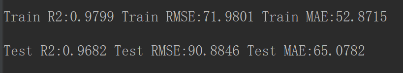
print("Train R2:%.4f" % sm.r2_score(y_train, pred_train))
print("Train RMSE:%.4f" % (sm.mean_squared_error(y_train, pred_train) ** 0.5))
print("Train MAE:%.4f" % (sm.mean_absolute_error(y_train, pred_train)))
print("Test R2:%.4f" % sm.r2_score(y_test, pred_test))
print("Test RMSE:%.4f" % (sm.mean_squared_error(y_test, pred_test) ** 0.5))
print("Test MAE:%.4f" % (sm.mean_absolute_error(y_test, pred_test)))

测试集预测结果可视化

# 20. 画密度图使用该库。
from scipy.stats import gaussian_kde

pred_test = np.array(pred_test).reshape(-1)
y_test = np.array(y_test).reshape(-1)
xy = np.vstack([pred_test, y_test])
z1 = gaussian_kde(xy)(xy)

pred_test_residual = np.array(y_test - pred_test).reshape(-1)
pred_test = np.array(pred_test).reshape(-1)
xy = np.vstack([pred_test, pred_test_residual])
z2 = gaussian_kde(xy)(xy)

fig = plt.figure(figsize=(10, 8), dpi=300)
gs = fig.add_gridspec(2, 1, hspace=0, wspace=0.2, left=0.13, top=0.98, bottom=0.1)
(ax1), (ax2) = gs.subplots(sharex='col')

ax11 = ax1.scatter(pred_test.tolist(), y_test.tolist(), s=2, c=z1)
ax1.plot([np.min(pred_test)-500, np.max(pred_test)+500], [np.min(pred_test)-500, np.max(pred_test)+500], "--", linewidth=1.5)
ax1.set_ylabel(r"$Test$", fontsize=25)
ax1.xaxis.set_major_locator(plt.MaxNLocator(3))
ax1.yaxis.set_major_locator(plt.MaxNLocator(4))
ax1.tick_params(top='on', right='on', which='both', labelsize=25)
ax1.set_xlim([np.min(pred_test)-500, np.max(pred_test)+500])
ax1.set_ylim([np.min(pred_test)-500, np.max(pred_test)+500])
ax1.xaxis.set_major_locator(plt.MultipleLocator(1000))
ax1.yaxis.set_major_locator(plt.MultipleLocator(1000))
ax1.xaxis.set_minor_locator(plt.MultipleLocator(250))
ax1.yaxis.set_minor_locator(plt.MultipleLocator(250))

ax2.scatter(pred_test.tolist(), (y_test - pred_test).tolist(), s=2, c=z2)
ax2.plot([np.min(pred_train)-500, np.max(pred_train)+500], [0, 0], "--", linewidth=1.5)
ax2.set_title(r"$σT_{eff}=%.i$" % (np.var(y_test - pred_test) ** 0.5), fontsize=25)
ax2.set_xlabel(r"$Pred \ T_{eff}(k)$", fontsize=25)
ax2.set_ylabel(r"$Residual$", fontsize=25)
ax2.tick_params(top='on', right='on', which='both', labelsize=25)
ax2.xaxis.set_major_locator(plt.MultipleLocator(1000))
ax2.yaxis.set_major_locator(plt.MultipleLocator(400))
ax2.xaxis.set_minor_locator(plt.MultipleLocator(250))
ax2.yaxis.set_minor_locator(plt.MultipleLocator(100))

plt.rcParams['font.size'] = 25
fig.colorbar(ax11,
             label="Density",
             cax=fig.add_axes([0.92, 0.1, 0.02, 0.86]), ax=(ax1, ax2))
plt.show()

LightGBM模型特征重要性

LightGBM模型特征重要性：整个拟合过程中，各变量参与节点分裂次数占所有变量总分裂次数之比。
特征重要性排序可以结合天文特征做进一步分析，说明模型稳定性。

plt.style.use("ggplot")
plt.figure(dpi=300)
plt.rcParams['font.size'] = 18
importance = pd.DataFrame({"importance": np.round(clf.feature_importances_ / np.sum(clf.feature_importances_), 3),
                          "names": x_train.columns})
importance = importance.sort_values(by="importance", ascending=True)
plt.barh(y=importance["names"],
         width=importance["importance"], height=0.2)
for a, b, label in zip(importance["importance"], importance["names"], importance["names"]):
    plt.text(a+0.06, b, "%.1f" % (a*100) + "%", ha='center', va='center', fontsize=14)
plt.title(r"$T_{eff}$ Feature importance", fontsize=18)
plt.xlabel("Feature importance", fontsize=18)
plt.ylabel("Features", fontsize=18)
plt.xticks(fontsize=16)
plt.yticks(fontsize=20)
plt.xlim([0, 1])
plt.gca().xaxis.set_major_locator(plt.MaxNLocator(4))
plt.show()

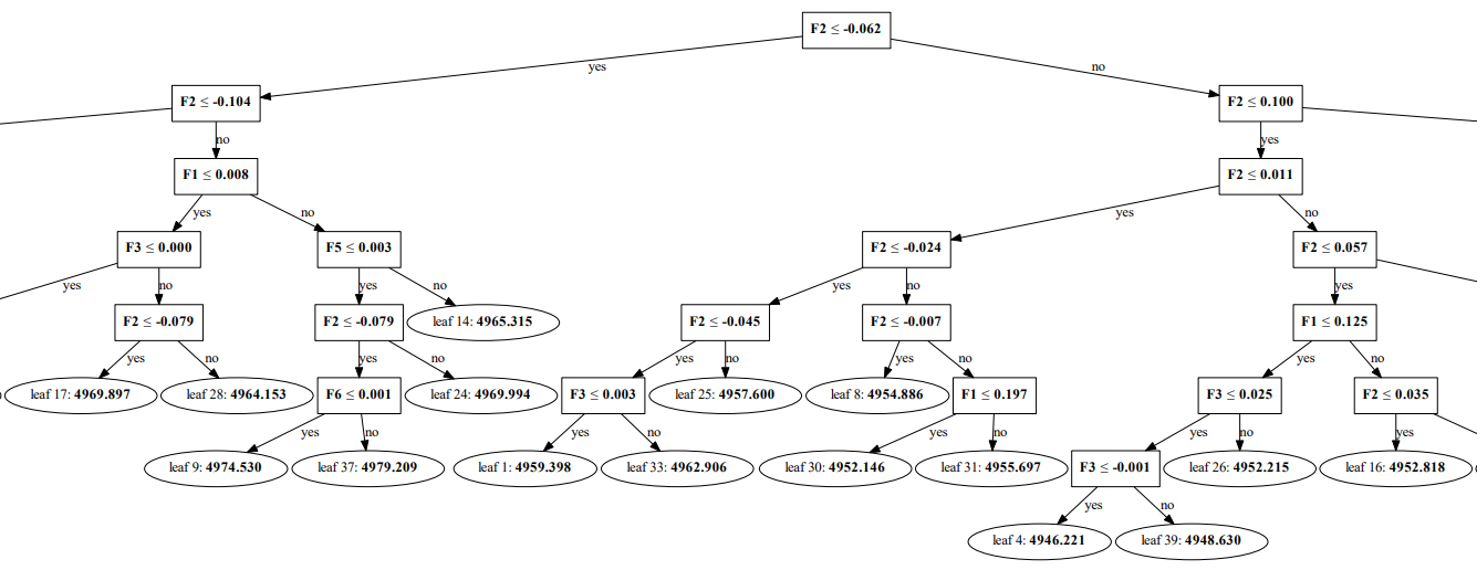
查看LightGBM模型任意一棵树

# 21. 查看第1棵树分裂模式。
dot_data = lgb.create_tree_digraph(clf, orientation="vertical", tree_index=0, name="tree1")
dot_data.format = 'PDF'
dot_data.render('TEFF_1.pdf')

LightGBM中GOSS的量化分析

范围取，其他参数取最优。如下图红点，当，时，误差最低。

# 22. 3维画图库。
from mpl_toolkits.mplot3d import Axes3D
from matplotlib import cm

RMSE = []
k = 12
A = np.linspace(0.01, 0.5, k)
B = np.linspace(0.01, 0.5, k)
for i in A:
    for j in B:
        clf = lgb.LGBMRegressor(objective='regression_l2',
                                random_state=666,
                                boosting_type="goss",
                                learning_rate=learning_rate,
                                max_depth=max_depth,
                                min_child_samples=min_child_samples,
                                n_estimators=n_estimators,
                                num_leaves=num_leaves,
                                subsample=subsample,
                                feature_fraction=feature_fraction,
                                lambda_l2=lambda_l2,
                                top_rate=i,
                                other_rate=j,
                                max_bin=max_bin,
                                importance_type="gain",
                                ).fit(x_train, y_train)
        pred_train = clf.predict(x_train)
        pred_test = clf.predict(x_test)

        RMSE.append(sm.mean_squared_error(y_test, pred_test) ** 0.5)
        print(i)
        print("Train R2:%.4f" % sm.r2_score(y_train, pred_train))
        print("Train RMSE:%.4f" % (sm.mean_squared_error(y_train, pred_train) ** 0.5))
        print("Train MAE:%.4f" % (sm.mean_absolute_error(y_train, pred_train)))
        print("Test R2:%.4f" % sm.r2_score(y_test, pred_test))
        print("Test RMSE:%.4f" % (sm.mean_squared_error(y_test, pred_test) ** 0.5))
        print("Test MAE:%.4f" % (sm.mean_absolute_error(y_test, pred_test)))

A, B = np.meshgrid(A, B)
RMSE = np.array(RMSE).reshape(k, k)
min_RMSE = np.argwhere(RMSE == np.min(RMSE))
min_A = A[min_RMSE[0][0], min_RMSE[0][1]]
min_B = B[min_RMSE[0][0], min_RMSE[0][1]]
min_RMSE = RMSE[min_RMSE[0][0], min_RMSE[0][1]]
print(min_A, min_B, min_RMSE)
fig, ax = plt.subplots(subplot_kw=dict(projection='3d'))
surf = ax.plot_surface(A, B, RMSE, cmap=cm.coolwarm, alpha=0.8)
ax.xaxis.set_major_locator(LinearLocator(5))
ax.yaxis.set_major_locator(LinearLocator(5))
ax.zaxis.set_major_locator(LinearLocator(5))
ax.xaxis.set_major_formatter(FormatStrFormatter('%.02f'))
ax.yaxis.set_major_formatter(FormatStrFormatter('%.02f'))
ax.zaxis.set_major_formatter(FormatStrFormatter('%.i'))
ax.set_xlabel(r'$a$', size=15)
ax.set_ylabel(r'$b$', size=15)
ax.set_xlim3d(0.01, 0.5)
ax.set_ylim3d(0.01, 0.5)
ax.set_zlim3d(88, 95)
ax.set_title("Influence of GOSS on Teff prediction RMSE", weight='bold', size=15)
fig.colorbar(surf, shrink=0.6, aspect=8, label="RMSE")
ax.scatter(min_A, min_B, min_RMSE, marker="o", c="r", s=20)
plt.show()

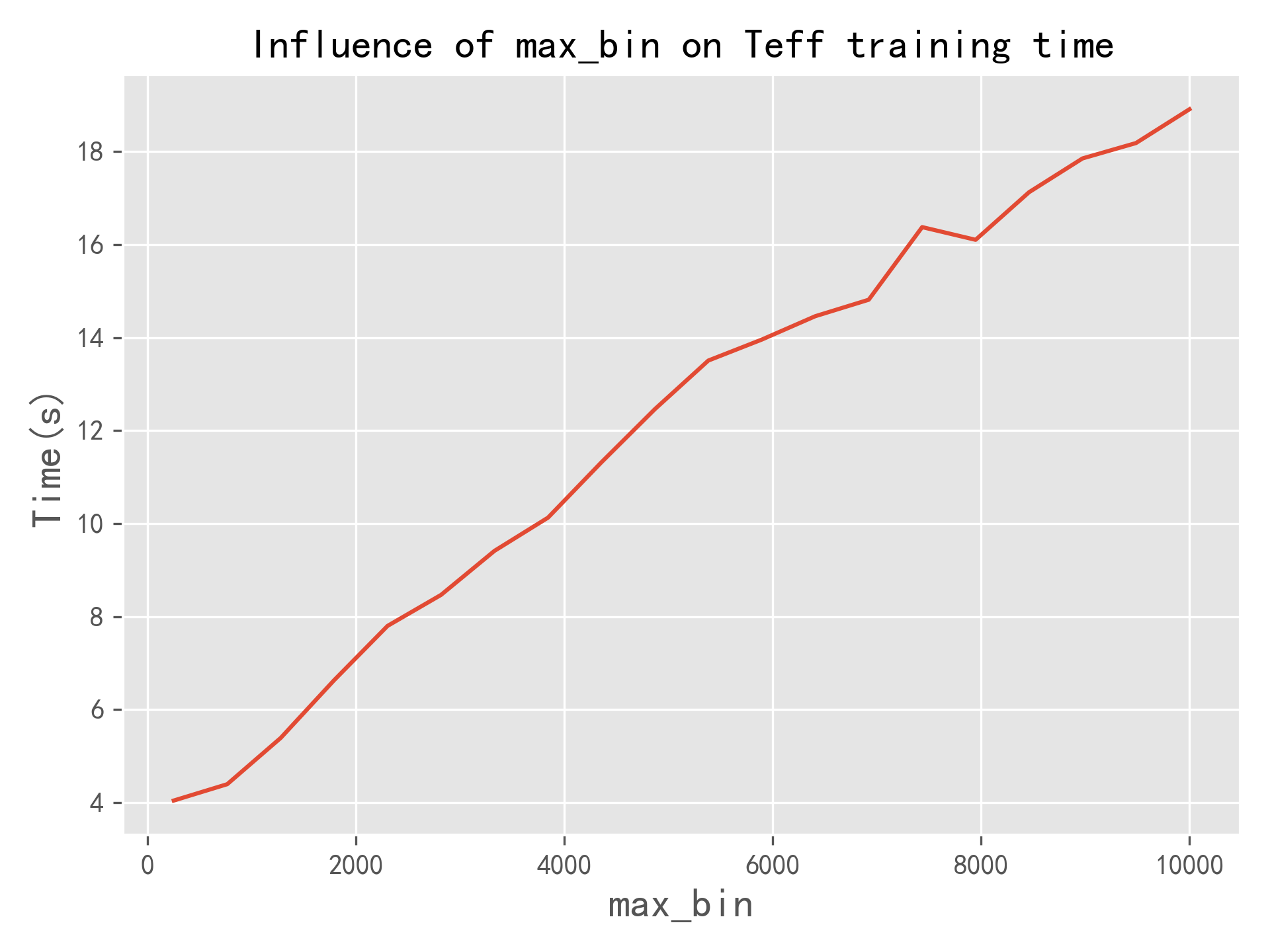
LightGBM中直方图方法的量化分析

箱子数量范围(s)为，步长，其他参数取最优。如下图所示，随着箱子数量增加，模型训练耗时线性增长。合适的s取值，是LIghtGBM模型更快的重要原因。

# 23. 计时库。
import time

RMSE = []
TIME = []
max_bin = np.linspace(250, 10000, 20)
print(max_bin)
for i in max_bin:
    time0 = time.time()
    clf = lgb.LGBMRegressor(objective='regression_l2',
                            random_state=666,
                            boosting_type="goss",
                            learning_rate=learning_rate,
                            max_depth=max_depth,
                            min_child_samples=min_child_samples,
                            n_estimators=n_estimators,
                            num_leaves=num_leaves,
                            subsample=subsample,
                            feature_fraction=feature_fraction,
                            lambda_l2=lambda_l2,
                            top_rate=top_rate,
                            other_rate=other_rate,
                            max_bin=int(i),
                            importance_type="gain",
                            ).fit(x_train, y_train)
    pred_train = clf.predict(x_train)
    pred_test = clf.predict(x_test)
    TIME.append(time.time() - time0)
    RMSE.append(sm.mean_squared_error(y_test, pred_test) ** 0.5)
    print(i)
    print("耗时", time.time() - time0)
    print("Train R2:%.4f" % sm.r2_score(y_train, pred_train))
    print("Train RMSE:%.4f" % (sm.mean_squared_error(y_train, pred_train) ** 0.5))
    print("Train MAE:%.4f" % (sm.mean_absolute_error(y_train, pred_train)))
    print("Test R2:%.4f" % sm.r2_score(y_test, pred_test))
    print("Test RMSE:%.4f" % (sm.mean_squared_error(y_test, pred_test) ** 0.5))
    print("Test MAE:%.4f" % (sm.mean_absolute_error(y_test, pred_test)))

plt.style.use("ggplot")
plt.figure(dpi=300)
plt.plot(max_bin, TIME)
plt.xlabel("max_bin", fontsize=15)
plt.ylabel("Time(s)", fontsize=15)
plt.title("Influence of max_bin on Teff training time", size=15)
plt.show()

LightGBM VS 部分机器学习模型

为了说明LightGBM模型的高性能，使用同样的数据集、贝叶斯优化方法对比随机森林、XGBoost、GBDT、ANN、SVR与线性回归在测试集中的预测结果。可以发现，LightGBM是一种更快速的模型，且泛化能力略强。因此，适应于大数据时代数据分析。

总结

主要讲述了LightGBM模型的原理以及在天文中的应用，原理部分参考Ke(2017)与Liang(2022)，天文应用部分取自Liang(2022)。
详细分析了LightGBM的GOSS与直方图带来的性能提升，GOSS主要提升模型泛化能力，直方图用于加速。
针对实验需求，没有讨论互斥特征捆绑(EFB)以及LightGBM按叶子生长策略，遗憾！

更多请参考 LightGBM: A Highly Efficient Gradient Boosting Decision Tree Guolin^[1]与Estimation of Stellar Atmospheric Parameters with Light Gradient Boosting Machine Algorithm and Principal Component Analysis^[2]