当前位置:网站首页>Deep understanding of Kalman filter (1): background knowledge
Deep understanding of Kalman filter (1): background knowledge
2022-07-27 08:51:00 【DeepDriving】
Deep understanding of Kalman filter (1): Background knowledge

Statement : The pictures and pictures of this article are from https://www.kalmanfilter.net/, If there is infringement, please contact to delete .
This article is from the official account of WeChat 【DeepDriving】 Arrangement , The full text is divided into 3 Part of it . Official account 【DeepDriving】, Background reply keyword 【 Kalman filter 】 The full text is available PDF.
Background knowledge
Before introducing the Kalman filter , Let's first learn some basic knowledge related to Mathematics .
Mean and expectation
mean value (Mean) And expectations (Expected Value) Are two similar but different concepts . If we have 2 gold 5 Penny and 3 gold 10 Cent coins , It's easy to calculate their mean :
V m e a n = 1 N ∑ n = 1 N V n = 1 5 ( 5 + 5 + 10 + 10 + 10 ) = 8 branch V_{mean}= \frac{1}{N} \sum _{n=1}^{N}V_{n}= \frac{1}{5} \left( 5+5+10+10+10 \right) = 8 branch Vmean=N1n=1∑NVn=51(5+5+10+10+10)=8 branch
The above results cannot be called expected values , Because the state of the system is not implicit and we use all 5 Coins to calculate the average .
Now suppose a person tests continuously 5 Secondary weight , The results are as follows :79.8 kg 、80 kg 、 80.1 kg 、79.8 kg 、80.2 kg , The random measurement error of the scale itself leads to different measurement values each time . We don't know what the real weight is , Because this is an implicit variable , But we can deal with 5 Calculate the average value of the measurement results of times to estimate a relatively accurate weight value :
W = 1 N ∑ n = 1 N W n = 1 5 ( 79.8 + 80 + 80.1 + 79.8 + 80.2 ) = 79.98 thousand g W= \frac{1}{N} \sum _{n=1}^{N}W_{n}= \frac{1}{5} \left( 79.8+80+80.1+79.8+80.2 \right) = 79.98 kg W=N1n=1∑NWn=51(79.8+80+80.1+79.8+80.2)=79.98 thousand g
The above average value can be called the expected value of implicit variable weight .
The average is usually written in Greek μ \mu μ To express , The expected value is written in letters E E E To express .
Variance and standard deviation
variance (Variance) Used to measure the dispersion of a set of data , That is, the deviation between the sample data and the mean ; Standard deviation (Standard Deviation) Is the square root of the variance , It's usually in Greek σ \sigma σ To express , And the variance is expressed as σ 2 \sigma^{2} σ2.
Suppose there are two high school basketball team members whose heights are shown in the following table :
| team member 1 | team member 2 | team member 3 | team member 4 | team member 5 | Average | |
|---|---|---|---|---|---|---|
| A team | 1.89m | 2.1m | 1.75m | 1.98m | 1.85m | 1.914m |
| B team | 1.94m | 1.9m | 1.97m | 1.89m | 1.87m | 1.914m |
We want to compare the height data of the two basketball teams . First , From the above table, we can know that the average height of the two teams is the same . Further , We can compare their variances and standard deviations . use x x x It means height , μ \mu μ Indicates the average height , According to the calculation formula of variance and standard deviation
σ 2 = 1 N ∑ n = 1 N ( x n − μ ) 2 \sigma ^{2}= \frac{1}{N} \sum _{n=1}^{N} \left( x_{n}- \mu \right) ^{2} σ2=N1n=1∑N(xn−μ)2
σ = 1 N ∑ n = 1 N ( x n − μ ) 2 \sigma =\sqrt[]{\frac{1}{N} \sum _{n=1}^{N} \left( x_{n}- \mu \right) ^{2}} σ=N1n=1∑N(xn−μ)2
Get A Variance of team height σ A 2 = 0.014 m 2 \sigma^{2}_{A}=0.014m^{2} σA2=0.014m2, Standard deviation σ A = 0.12 m \sigma_{A}=0.12m σA=0.12m;B Variance of team height σ B 2 = 0.0013 m 2 \sigma^{2}_{B}=0.0013m^{2} σB2=0.0013m2, Standard deviation σ B = 0.036 m \sigma_{B}=0.036m σB=0.036m. We can know from the variance of the height of the two teams ,A There is a greater difference in the height of team members .
Suppose we want to calculate the mean and variance of the height of all the players of all high school basketball teams , This will be a difficult task , Because we need to collect statistics from every team member in every school . However, we can collect a relatively large data set , Then the mean and variance of the height of all team members are estimated through this data set . such as , We can charge randomly 100 Height data of team members , This data set is enough to accurately estimate the mean and variance of the height of all team members . It should be noted that , At this time, the formula for calculating variance is slightly different from the above , Divisor is N − 1 N-1 N−1 instead of N N N:
σ 2 = 1 N − 1 ∑ n = 1 N ( x n − μ ) 2 \sigma ^{2}= \frac{1}{N-1} \sum _{n=1}^{N} \left( x_{n}- \mu \right) ^{2} σ2=N−11n=1∑N(xn−μ)2
coefficient N − 1 N-1 N−1 It is called Bessel correction (Bessel's correction), For detailed mathematical proof, please refer to This article .
Normal distribution
Many natural phenomena follow normal distribution (Normal Distribution) Laws . Take the height of basketball players as an example , If we randomly select the height of the team members to build a large data set , And draw a graph of height value and its occurrence frequency , We will get a bell curve similar to the figure below :

You can see that this curve is based on the mean 1.9m A symmetrical curve centered , And the number of occurrences of values near the mean value is much higher than that of remote values . The standard deviation of this set of data is 0.2m, As shown in the figure below , Yes 68.26% The value of is within one standard deviation from the mean (1.7m~2.1m):

Normal distribution is also called Gaussian distribution , The formula is as follows :
f ( x ; μ , σ 2 ) = 1 2 π σ 2 e − ( x − μ ) 2 2 σ 2 f \left( x; \mu , \sigma ^{2} \right) = \frac{1}{\sqrt[]{2 \pi \sigma ^{2}}}e^{\frac{- \left( x- \mu \right) ^{2}}{2 \sigma ^{2}}} f(x;μ,σ2)=2πσ21e2σ2−(x−μ)2
The above curve is called the probability density function of normal distribution (Probability Density Function,PDF).
The measurement error usually conforms to the normal distribution , Therefore, when designing Kalman filter, we will assume that the measurement error is normally distributed .
A random variable
If you use a speed gun to measure the speed of a moving vehicle , Then the measured value of the velocimeter gun is a random variable , The measurement results are normally distributed . Random variables can be continuous , It can also be discrete , All measurements are continuous random variables .
It is estimated that 、 Accuracy and accuracy
It is estimated that (Estimate) It is an estimation of the implicit state of the system . For example, the real position of the aircraft is an implicit state value for the observer , We can use radar and other sensors to measure and improve the accuracy of estimation through multi-sensor fusion and tracking algorithm . The measured or calculated parameters are estimated values .
Accuracy (Accuracy) Used to indicate the closeness between the measured value and the real value .
accuracy (Precision) Used to express the reproducibility of measurement results .
Estimation needs to consider the accuracy and accuracy of the system , The following figure illustrates the relationship between accuracy and precision :

The variance of the measured value of the high-precision system is small ( Low uncertainty ), conversely , The variance of the measured value of the low accuracy system is large ( High uncertainty ), Variance is caused by random measurement error .
Systems with low accuracy are called biased systems , Because there will always be an internal systematic error in its measured value ( deviation ).
Averaging or smoothing the measured values can significantly reduce the influence of variance . such as , If we use a thermometer with random measurement error to measure temperature , Measurement error will cause the measured value to be higher or lower than the true value . We can make multiple measurements and average them , This estimate will be close to the real value , The more measurements , The closer the estimated value is to the real value . But if the thermometer itself has deviation , Then the estimated value will have a fixed systematic error .
The following figure describes the measured values from a statistical point of view :

- The measured value is a random variable described by the probability density function ;
- The mean value of the measured value is the expected value of the random variable ;
- The deviation between the mean value of the measured value and the true value is called deviation or systematic measurement error , Used to indicate the accuracy of measurement ;
- The degree of dispersion of the measured value distribution is the accuracy of the measured value , Also known as measurement noise (
measurement noise)、 Random measurement error (random measurement error) Or measurement uncertainty (measurement uncertainty).
Covariance and covariance matrix
Covariance is used to measure two random variables x x x and y y y The degree of joint change , It represents the overall error of two variables , This is different from variance , Variance represents only one variable error . Variance can be regarded as a special case of covariance , That is, the two variables are the same . If the trends of the two variables are the same , That is, if one of them is greater than its own expectations , The other is also greater than one's own expectations , Then the covariance between the two variables is positive . If the change trend of two variables is opposite , That is, one of them is greater than its own expectation , And the other is less than its own expectations , Then the covariance between the two variables is negative . If x x x And y y y It's statistically independent , So the covariance between them is going to be 0. A random variable x x x And y y y The covariance of is calculated as follows :
σ ( x , y ) = 1 N − 1 ∑ n = 1 N ( x n − μ x ) ( y n − μ y ) \sigma(x,y)= \frac{1}{N-1} \sum _{n=1}^{N} \left( x_{n}- \mu_{x} \right) \left( y_{n}- \mu_{y} \right) σ(x,y)=N−11n=1∑N(xn−μx)(yn−μy)
among , μ x \mu_{x} μx and μ y \mu_{y} μy They are random variables x x x And y y y Average value .
For a sample containing k k k Vectors of elements x \boldsymbol{x} x
[ x 1 x 2 x 3 … x k ] T \begin{bmatrix} x_{1} & x_{2} & x_{3} & \dots & x_{k} \end{bmatrix}^{T} [x1x2x3…xk]T
The covariance matrix is
C O V ( x ) = E ( [ ( x 1 − μ x 1 ) 2 ( x 1 − μ x 1 ) ( x 2 − μ x 2 ) ⋯ ( x 1 − μ x 1 ) ( x k − μ x k ) ( x 2 − μ x 2 ) ( x 1 − μ x 1 ) ( x 2 − μ x 2 ) 2 ⋯ ( x 2 − μ x 2 ) ( x k − μ x k ) ⋮ ⋮ ⋱ ⋮ ( x k − μ x k ) ( x 1 − μ x 1 ) ( x k − μ x k ) ( x 2 − μ x 2 ) ⋯ ( x k − μ x k ) 2 ] ) = E ( [ ( x 1 − μ x 1 ) ( x 2 − μ x 2 ) ⋮ ( x k − μ x k ) ] [ ( x 1 − μ x 1 ) ( x 2 − μ x 2 ) ⋯ ( x k − μ x k ) ] ) = E ( ( x − μ x ) ( x − μ x ) T ) COV(\boldsymbol{x}) = E\left( \left[ \begin{matrix} (x_{1} - \mu_{x_{1}})^{2} & (x_{1} - \mu_{x_{1}})(x_{2} - \mu_{x_{2}}) & \cdots & (x_{1} - \mu_{x_{1}})(x_{k} - \mu_{x_{k}}) \\ (x_{2} - \mu_{x_{2}})(x_{1} - \mu_{x_{1}}) & (x_{2} - \mu_{x_{2}})^{2} & \cdots & (x_{2} - \mu_{x_{2}})(x_{k} - \mu_{x_{k}}) \\ \vdots & \vdots & \ddots & \vdots \\ (x_{k} - \mu_{x_{k}})(x_{1} - \mu_{x_{1}}) & (x_{k} - \mu_{x_{k}})(x_{2} - \mu_{x_{2}}) & \cdots & (x_{k} - \mu_{x_{k}})^{2} \\ \end{matrix} \right] \right) \\ = E\left( \left[ \begin{matrix} (x_{1} - \mu_{x_{1}}) \\ (x_{2} - \mu_{x_{2}}) \\ \vdots \\ (x_{k} - \mu_{x_{k}}) \\ \end{matrix} \right] \left[ \begin{matrix} (x_{1} - \mu_{x_{1}}) & (x_{2} - \mu_{x_{2}}) & \cdots & (x_{k} - \mu_{x_{k}}) \end{matrix} \right] \right) \\ = E\left( \left( \boldsymbol{x - \mu_{x}} \right) \left( \boldsymbol{x - \mu_{x}} \right)^{T} \right) COV(x)=E⎝⎜⎜⎜⎛⎣⎢⎢⎢⎡(x1−μx1)2(x2−μx2)(x1−μx1)⋮(xk−μxk)(x1−μx1)(x1−μx1)(x2−μx2)(x2−μx2)2⋮(xk−μxk)(x2−μx2)⋯⋯⋱⋯(x1−μx1)(xk−μxk)(x2−μx2)(xk−μxk)⋮(xk−μxk)2⎦⎥⎥⎥⎤⎠⎟⎟⎟⎞=E⎝⎜⎜⎜⎛⎣⎢⎢⎢⎡(x1−μx1)(x2−μx2)⋮(xk−μxk)⎦⎥⎥⎥⎤[(x1−μx1)(x2−μx2)⋯(xk−μxk)]⎠⎟⎟⎟⎞=E((x−μx)(x−μx)T)
Basic expectation operation rules
A random variable X X X The expectations of the E ( X ) E(X) E(X) Equal to its average :
E ( X ) = μ X E(X) = \mu_{X} E(X)=μX
Some basic expectation operation rules are as follows :
| The rules | remarks |
|---|---|
| E ( X ) = μ X = ∑ x p ( x ) E(X) = \mu_{X}=\sum{xp(x)} E(X)=μX=∑xp(x) | p ( x ) p(x) p(x) yes x x x Probability |
| E ( a ) = a E(a) = a E(a)=a | a a a Constant |
| E ( a X ) = a E ( X ) E(aX) = aE(X) E(aX)=aE(X) | a a a Constant |
| E ( a ± X ) = a ± E ( X ) E(a\pm{X}) = a\pm{E(X)} E(a±X)=a±E(X) | a a a Constant |
| E ( a ± b X ) = a ± b E ( X ) E(a\pm{bX}) = a\pm{bE(X)} E(a±bX)=a±bE(X) | a , b a,b a,b Constant |
| E ( X ± Y ) = E ( X ) ± E ( Y ) E(X\pm{Y}) = E(X)\pm{E(Y)} E(X±Y)=E(X)±E(Y) | Y Y Y For another random variable |
| E ( X Y ) = E ( X ) E ( Y ) E(XY) = E(X)E(Y) E(XY)=E(X)E(Y) | If X X X and Y Y Y Are independent of each other |
The random variable X X X and Y Y Y The variances of are recorded as V ( X ) V(X) V(X) and V ( Y ) V(Y) V(Y), Their covariance is recorded as C O V ( X , Y ) COV(X,Y) COV(X,Y), Here are some basic operation rules :
| The rules | remarks |
|---|---|
| V ( a ) = 0 V(a)=0 V(a)=0 | a a a Constant |
| V ( a ± X ) = V ( X ) V(a\pm{X})=V(X) V(a±X)=V(X) | a a a Constant |
| V ( X ) = E ( X 2 ) − μ X 2 V(X)=E(X^{2})-\mu^{2}_{X} V(X)=E(X2)−μX2 | |
| C O V ( X , Y ) = E ( X Y ) − μ X μ Y COV(X,Y)=E(XY)-\mu_{X}\mu_{Y} COV(X,Y)=E(XY)−μXμY | |
| C O V ( X , Y ) = 0 COV(X,Y)=0 COV(X,Y)=0 | If X X X and Y Y Y Are independent of each other |
| V ( a X ) = a 2 V ( X ) V(aX) = a^{2}V(X) V(aX)=a2V(X) | a a a Constant |
| V ( X ± Y ) = V ( X ) + V ( Y ) ± 2 C O V ( X , Y ) V(X\pm{Y}) = V(X)+V(Y)\pm{2COV(X,Y)} V(X±Y)=V(X)+V(Y)±2COV(X,Y) | |
| V ( X Y ) ≠ V ( X ) V ( Y ) V(XY) \ne V(X)V(Y) V(XY)=V(X)V(Y) |
The following is the proof of several formulas :
(1).
V ( X ) = E ( ( X − μ X ) 2 ) = E ( X 2 − 2 X μ X + μ X 2 ) = E ( X 2 ) − E ( 2 X μ X ) + E ( μ X 2 ) = E ( X 2 ) − 2 μ X E ( X ) + μ X 2 = E ( X 2 ) − 2 μ X μ X + μ X 2 = E ( X 2 ) − μ X 2 V(X) = E((X-\mu_{X})^{2}) \\ = E(X^{2}-2X\mu_{X}+\mu^{2}_{X}) \\ = E(X^{2})-E(2X\mu_{X})+E(\mu^{2}_{X}) \\ = E(X^{2})-2\mu_{X}E(X)+\mu^{2}_{X} \\ = E(X^{2})-2\mu_{X}\mu_{X}+\mu^{2}_{X} \\ = E(X^{2})-\mu^{2}_{X} \\ V(X)=E((X−μX)2)=E(X2−2XμX+μX2)=E(X2)−E(2XμX)+E(μX2)=E(X2)−2μXE(X)+μX2=E(X2)−2μXμX+μX2=E(X2)−μX2
(2).
C O V ( X ) = E ( ( X − μ X ) ( Y − μ Y ) ) = E ( X Y − X μ Y − Y μ X + μ X μ Y ) = E ( X Y ) − E ( X μ Y ) − E ( Y μ X ) + E ( μ X μ Y ) = E ( X Y ) − μ Y E ( X ) − μ X E ( Y ) + E ( μ X μ Y ) = E ( X Y ) − μ Y μ X − μ X μ Y + μ X μ Y = E ( X Y ) − μ X μ Y COV(X) = E((X-\mu_{X})(Y-\mu_{Y})) \\ = E(XY - X \mu_{Y} - Y \mu_{X} + \mu_{X}\mu_{Y}) \\ = E(XY) - E(X \mu_{Y}) - E(Y \mu_{X}) + E(\mu_{X}\mu_{Y}) \\ = E(XY) - \mu_{Y} E(X) - \mu_{X} E(Y) + E(\mu_{X}\mu_{Y}) \\ = E(XY) - \mu_{Y} \mu_{X} - \mu_{X} \mu_{Y} + \mu_{X}\mu_{Y} \\ = E(XY) - \mu_{X}\mu_{Y} \\ COV(X)=E((X−μX)(Y−μY))=E(XY−XμY−YμX+μXμY)=E(XY)−E(XμY)−E(YμX)+E(μXμY)=E(XY)−μYE(X)−μXE(Y)+E(μXμY)=E(XY)−μYμX−μXμY+μXμY=E(XY)−μXμY
(3).
V ( a X ) = E ( ( a X ) 2 ) − ( a μ X ) 2 = E ( a 2 X 2 ) − a 2 μ X 2 = a 2 E ( X 2 ) − a 2 μ X 2 = a 2 ( E ( X 2 ) − μ X 2 ) = a 2 V ( X ) V(aX) = E((aX)^{2})-(a\mu_{X})^{2} \\ = E(a^{2}X^{2})-a^{2}\mu_{X}^{2} \\ = a^{2}E(X^{2})-a^{2}\mu_{X}^{2} \\ = a^{2}(E(X^{2})-\mu_{X}^{2}) \\ = a^{2}V(X) \\ V(aX)=E((aX)2)−(aμX)2=E(a2X2)−a2μX2=a2E(X2)−a2μX2=a2(E(X2)−μX2)=a2V(X)
(4).
V ( X ± Y ) = E ( ( X ± Y ) 2 ) − ( μ X ± μ Y ) 2 = E ( X 2 ± 2 X Y + Y 2 ) − ( μ X 2 ± 2 μ X μ Y + μ y 2 ) = E ( X 2 ) − μ X 2 + E ( Y 2 ) − μ Y 2 ± 2 ( E ( X Y ) − μ X μ Y ) = V ( X ) + V ( Y ) ± 2 ( E ( X Y ) − μ X μ Y ) = V ( X ) + V ( Y ) ± 2 C O V ( X , Y ) V(X\pm{Y}) = E((X \pm Y)^{2}) - (\mu_{X} \pm \mu_{Y})^{2} \\ = E(X^{2} \pm 2XY + Y^{2}) - (\mu_{X}^2 \pm 2\mu_{X}\mu_{Y} + \mu_{y}^2) \\ = {E(X^{2}) - \mu_{X}^2} + {E(Y^{2}) - \mu_{Y}^2} \pm 2(E(XY) - \mu_{X}\mu_{Y} ) \\ = {V(X)} + {V(Y)} \pm 2(E(XY) - \mu_{X}\mu_{Y} ) \\ = V(X) + V(Y) \pm 2COV(X,Y) \\ V(X±Y)=E((X±Y)2)−(μX±μY)2=E(X2±2XY+Y2)−(μX2±2μXμY+μy2)=E(X2)−μX2+E(Y2)−μY2±2(E(XY)−μXμY)=V(X)+V(Y)±2(E(XY)−μXμY)=V(X)+V(Y)±2COV(X,Y)
Differential of matrix product trace
Here we will prove two formulas .
(1).
d d A ( t r ( A B ) ) = B T \frac{d}{d\boldsymbol{A}} \left( tr\left( \boldsymbol{AB} \right) \right) = \boldsymbol{B}^{T} dAd(tr(AB))=BT
prove :
Given two matrices A \boldsymbol{A} A( m × n m\times n m×n) and B \boldsymbol{B} B( n × m n\times m n×m), The product of them is
A B = [ a 11 ⋯ a 1 n ⋮ ⋱ ⋮ a m 1 ⋯ a m n ] [ b 11 ⋯ b 1 m ⋮ ⋱ ⋮ b n 1 ⋯ b n m ] = [ ∑ i = 1 n a 1 i b i 1 ⋯ ∑ i = 1 n a 1 i b i m ⋮ ⋱ ⋮ ∑ i = 1 n a m i b i 1 ⋯ ∑ i = 1 n a m i b i m ] \boldsymbol{AB}= \left[ \begin{matrix} a_{11} & \cdots & a_{1n} \\ \vdots & \ddots & \vdots \\ a_{m1} & \cdots & a_{mn} \\ \end{matrix} \right] \left[ \begin{matrix} b_{11} & \cdots & b_{1m} \\ \vdots & \ddots & \vdots \\ b_{n1} & \cdots & b_{nm} \\ \end{matrix} \right] = \left[ \begin{matrix} \sum_{i=1}^{n}a_{1i}b_{i1} & \cdots & \sum_{i=1}^{n}a_{1i}b_{im} \\ \vdots & \ddots & \vdots \\ \sum_{i=1}^{n}a_{mi}b_{i1} & \cdots & \sum_{i=1}^{n}a_{mi}b_{im} \\ \end{matrix} \right] AB=⎣⎢⎡a11⋮am1⋯⋱⋯a1n⋮amn⎦⎥⎤⎣⎢⎡b11⋮bn1⋯⋱⋯b1m⋮bnm⎦⎥⎤=⎣⎢⎡∑i=1na1ibi1⋮∑i=1namibi1⋯⋱⋯∑i=1na1ibim⋮∑i=1namibim⎦⎥⎤
matrix A B \boldsymbol{AB} AB The trace of t r ( A B ) tr(\boldsymbol{AB}) tr(AB) Is the sum of its main diagonal elements :
t r ( A B ) = ∑ i = 1 n a 1 i b i 1 + ⋯ + ∑ i = 1 n a m i b i m = ∑ i = 1 n ∑ j = 1 m a j i b i j tr(\boldsymbol{AB}) = \sum_{i=1}^{n}a_{1i}b_{i1} + \cdots + \sum_{i=1}^{n}a_{mi}b_{im} = \sum_{i=1}^{n}\sum_{j=1}^{m}a_{ji}b_{ij} tr(AB)=i=1∑na1ibi1+⋯+i=1∑namibim=i=1∑nj=1∑majibij
Contralateral trace t r ( A B ) tr(\boldsymbol{AB}) tr(AB) Find differentiation
∂ t r ( A B ) ∂ A = [ ∂ ( ∑ i = 1 n ∑ j = 1 m a j i b i j ) ∂ a 11 ⋯ ∂ ( ∑ i = 1 n ∑ j = 1 m a j i b i j ) ∂ a 1 n ⋮ ⋱ ⋮ ∂ ( ∑ i = 1 n ∑ j = 1 m a j i b i j ) ∂ a m 1 ⋯ ∂ ( ∑ i = 1 n ∑ j = 1 m a j i b i j ) ∂ a m n ] = [ b 11 ⋯ b n 1 ⋮ ⋱ ⋮ b 1 m ⋯ b n m ] = B T \frac{\partial tr(\boldsymbol{AB})}{\partial\boldsymbol{A}} = \left[ \begin{matrix} \frac{\partial (\sum_{i=1}^{n}\sum_{j=1}^{m}a_{ji}b_{ij})}{\partial a_{11}} & \cdots & \frac{\partial (\sum_{i=1}^{n}\sum_{j=1}^{m}a_{ji}b_{ij})}{\partial a_{1n}} \\ \vdots & \ddots & \vdots \\ \frac{\partial (\sum_{i=1}^{n}\sum_{j=1}^{m}a_{ji}b_{ij})}{\partial a_{m1}} & \cdots & \frac{\partial (\sum_{i=1}^{n}\sum_{j=1}^{m}a_{ji}b_{ij})}{\partial a_{mn}} \\ \end{matrix} \right] \\ = \left[ \begin{matrix} b_{11} & \cdots & b_{n1} \\ \vdots & \ddots & \vdots \\ b_{1m} & \cdots & b_{nm} \\ \end{matrix} \right] \\ = \boldsymbol{B}^{T} ∂A∂tr(AB)=⎣⎢⎢⎡∂a11∂(∑i=1n∑j=1majibij)⋮∂am1∂(∑i=1n∑j=1majibij)⋯⋱⋯∂a1n∂(∑i=1n∑j=1majibij)⋮∂amn∂(∑i=1n∑j=1majibij)⎦⎥⎥⎤=⎣⎢⎡b11⋮b1m⋯⋱⋯bn1⋮bnm⎦⎥⎤=BT
(2).
d d A ( t r ( A B A T ) ) = 2 A B \frac{d}{d\boldsymbol{A}} \left( tr\left( \boldsymbol{ABA^{T}} \right) \right) = 2\boldsymbol{AB} dAd(tr(ABAT))=2AB
among B \boldsymbol{B} B Is symmetric matrix .
prove :
Given two matrices A \boldsymbol{A} A( m × n m\times n m×n) and B \boldsymbol{B} B( n × m n\times m n×m),
A B A T = [ a 11 ⋯ a 1 n ⋮ ⋱ ⋮ a m 1 ⋯ a m n ] [ b 11 ⋯ b 1 n ⋮ ⋱ ⋮ b n 1 ⋯ b n n ] [ a 11 ⋯ a m 1 ⋮ ⋱ ⋮ a 1 n ⋯ a m n ] = ( [ ∑ i = 1 n a 1 i b i 1 ⋯ ∑ i = 1 n a 1 i b i n ⋮ ⋱ ⋮ ∑ i = 1 n a m i b i 1 ⋯ ∑ i = 1 n a m i b i n ] ) [ a 11 ⋯ a m 1 ⋮ ⋱ ⋮ a 1 n ⋯ a m n ] = [ ∑ j = 1 n ∑ i = 1 n a 1 i b i j a 1 j ⋯ ∑ j = 1 n ∑ i = 1 n a 1 i b i j a m j ⋮ ⋱ ⋮ ∑ j = 1 n ∑ i = 1 n a m i b i j a 1 j ⋯ ∑ j = 1 n ∑ i = 1 n a m i b i j a m j ] \boldsymbol{ABA}^{T} = \left[ \begin{matrix} a_{11} & \cdots & a_{1n} \\ \vdots & \ddots & \vdots \\ a_{m1} & \cdots & a_{mn} \\ \end{matrix} \right] \left[ \begin{matrix} b_{11} & \cdots & b_{1n} \\ \vdots & \ddots & \vdots \\ b_{n1} & \cdots & b_{nn} \\ \end{matrix} \right] \left[ \begin{matrix} a_{11} & \cdots & a_{m1} \\ \vdots & \ddots & \vdots \\ a_{1n} & \cdots & a_{mn} \\ \end{matrix} \right] \\ = \left( \left[ \begin{matrix} \sum_{i=1}^{n}a_{1i}b_{i1} & \cdots & \sum_{i=1}^{n}a_{1i}b_{in} \\ \vdots & \ddots & \vdots \\ \sum_{i=1}^{n}a_{mi}b_{i1} & \cdots & \sum_{i=1}^{n}a_{mi}b_{in} \\ \end{matrix} \right] \right) \left[ \begin{matrix} a_{11} & \cdots & a_{m1} \\ \vdots & \ddots & \vdots \\ a_{1n} & \cdots & a_{mn} \\ \end{matrix} \right] \\ = \left[ \begin{matrix} \sum_{j=1}^{n}\sum_{i=1}^{n}a_{1i}b_{ij}a_{1j} & \cdots & \sum_{j=1}^{n}\sum_{i=1}^{n}a_{1i}b_{ij}a_{mj} \\ \vdots & \ddots & \vdots \\ \sum_{j=1}^{n}\sum_{i=1}^{n}a_{mi}b_{ij}a_{1j} & \cdots & \sum_{j=1}^{n}\sum_{i=1}^{n}a_{mi}b_{ij}a_{mj} \\ \end{matrix} \right] \\ ABAT=⎣⎢⎡a11⋮am1⋯⋱⋯a1n⋮amn⎦⎥⎤⎣⎢⎡b11⋮bn1⋯⋱⋯b1n⋮bnn⎦⎥⎤⎣⎢⎡a11⋮a1n⋯⋱⋯am1⋮amn⎦⎥⎤=⎝⎜⎛⎣⎢⎡∑i=1na1ibi1⋮∑i=1namibi1⋯⋱⋯∑i=1na1ibin⋮∑i=1namibin⎦⎥⎤⎠⎟⎞⎣⎢⎡a11⋮a1n⋯⋱⋯am1⋮amn⎦⎥⎤=⎣⎢⎡∑j=1n∑i=1na1ibija1j⋮∑j=1n∑i=1namibija1j⋯⋱⋯∑j=1n∑i=1na1ibijamj⋮∑j=1n∑i=1namibijamj⎦⎥⎤
matrix A B A T \boldsymbol{ABA}^{T} ABAT The trace of t r ( A B A T ) tr(\boldsymbol{ABA}^{T}) tr(ABAT) Is the sum of its main diagonal elements :
t r ( A B A T ) = ∑ j = 1 n ∑ i = 1 n a 1 i b i j a 1 j + ⋯ + ∑ j = 1 n ∑ i = 1 n a m i b i j a m j = ∑ k = 1 m ∑ j = 1 n ∑ i = 1 n a k i b i j a k j tr(\boldsymbol{ABA}^{T}) = \sum_{j=1}^{n}\sum_{i=1}^{n}a_{1i}b_{ij}a_{1j} + \cdots + \sum_{j=1}^{n}\sum_{i=1}^{n}a_{mi}b_{ij}a_{mj} = \sum_{k=1}^{m}\sum_{j=1}^{n}\sum_{i=1}^{n}a_{ki}b_{ij}a_{kj} tr(ABAT)=j=1∑ni=1∑na1ibija1j+⋯+j=1∑ni=1∑namibijamj=k=1∑mj=1∑ni=1∑nakibijakj
Contralateral trace t r ( A B A T ) tr(\boldsymbol{ABA}^{T}) tr(ABAT) Find differentiation 
Because the matrix B \boldsymbol{B} B It's a symmetric matrix , therefore B = B T \boldsymbol{B=B^{T}} B=BT, Available
∂ t r ( A B A T ) ∂ A = A B T + A B = A B + A B = 2 A B \frac{\partial tr(\boldsymbol{ABA}^{T})}{\partial\boldsymbol{A}} = \boldsymbol{AB}^{T} + \boldsymbol{AB} = \boldsymbol{AB} + \boldsymbol{AB} = 2\boldsymbol{AB} ∂A∂tr(ABAT)=ABT+AB=AB+AB=2AB
边栏推荐
- Create a project to realize login and registration, generate JWT, and send verification code
- 4277. Block reversal
- Cookie addition, deletion, modification and exception
- 微信安装包从0.5M暴涨到260M,为什么我们的程序越来越大?
- Arm undefined instruction exception assembly
- NIO示例
- MySQL basic knowledge learning (I)
- Matlab数据导入--importdata和load函数
- Cenos7 update MariaDB
- User management - restrictions
猜你喜欢

How to merge multiple columns in an excel table into one column

Network IO summary

Unity3D 2021软件安装包下载及安装教程
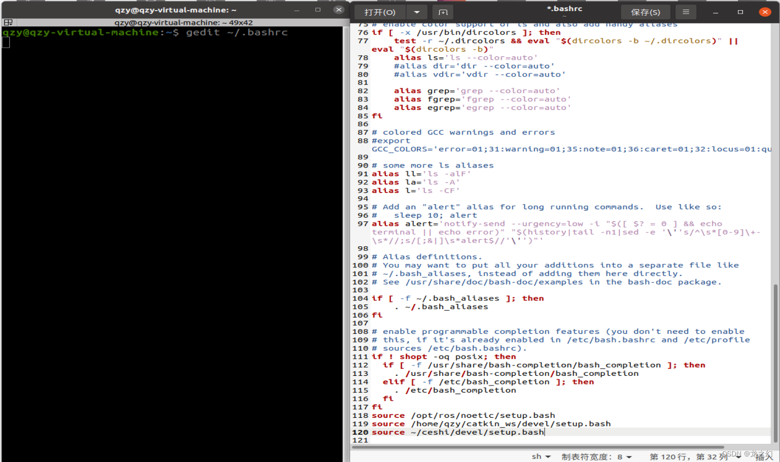
永久设置source的方法

08_ Service fusing hystrix

Arm system call exception assembly

4274. Suffix expression

E. Split into two sets
![ROS2安装时出现Connection failed [IP: 91.189.91.39 80]](/img/7f/92b7d44cddc03c58364d8d3f19198a.png)
ROS2安装时出现Connection failed [IP: 91.189.91.39 80]
NiO Summary - read and understand the whole NiO process
随机推荐
691. Cube IV
redis的string类型及bitmap
Implementation of registration function
Matlab drawing skills and examples: stackedplot
Solve the problem of Chinese garbled code on the jupyter console
Background coupon management
N queen problem (backtracking, permutation tree)
数智革新
Hangzhou E-Commerce Research Institute released an explanation of the new term "digital existence"
List delete collection elements
Include error in vs Code (new header file)
Sequential storage and chain storage of stack implementation
永久设置source的方法
Can "Gulangyu yuancosmos" become an "upgraded sample" of China's cultural tourism industry
How to merge multiple columns in an excel table into one column
4278. Summit
【进程间通信IPC】- 信号量的学习
接口测试工具-Jmeter压力测试使用
Encountered 7 file(s) that should have been pointers, but weren‘t
New year's goals! The code is more standardized!