当前位置:网站首页>Master go game through deep neural network and tree search
Master go game through deep neural network and tree search
2022-07-08 02:07:00 【Wwwilling】
Article
author :David Silver*, Aja Huang*, Chris J. Maddison etc.
Literature title : Master the go game through deep neural network and tree search
Document time :2016
Journal Publishing :nature
https://github.com/jmgilmer/GoCNN
Abstract
Due to its huge search space and the difficulty of evaluating the position and movement of the chessboard , Go has always been regarded as the most challenging game in the classic AI Games . ad locum , We introduce a new method of computer go , It USES “ Value network ” To evaluate the chessboard position and “ Policy network ” To choose how to walk . These deep neural networks are trained through a novel combination of supervised learning of human expert games and reinforcement learning of self Games . Without any forward-looking search , Neural networks play go at the level of the most advanced Monte Carlo tree search program , Simulate thousands of random self Games . We also introduce a new search algorithm , It combines Monte Carlo simulation with value and strategy Networks . Use this search algorithm , Our program AlphaGo Other go programs have achieved 99.8% Winning rate , With 5 Than 0 Defeated the human European go champion . This is the first time that computer programs have completely defeated human professional chess player go , It used to be thought that it would take at least ten years to achieve this feat .
All perfect information games have an optimal value function v ∗ ( s ) v^*(s) v∗(s), It determines that when all players play perfectly , Each chessboard position or state s s s The result of the game . These games can be played by including about b d b^d bd Recursively calculate the optimal value function in the search tree of a possible moving sequence to solve , among b b b Is the breadth of the game ( Number of legal moves per location ), d d d Is its depth ( Game length ). In a big game , For example, chess ( b ≈ 35 , d ≈ 80 ) (b≈35,d≈80) (b≈35,d≈80), Especially go ( b ≈ 250 , d ≈ 150 ) (b≈250,d≈150) (b≈250,d≈150), Exhaustive search is not feasible , But there are two general principles to reduce the effective search space . First , The depth of search can be reduced by location evaluation : Truncation state s s s Search tree at , And use an approximation function v ( s ) ≈ v ∗ ( s ) v(s)≈v^*(s) v(s)≈v∗(s) Replace s s s The subtree below , This function can predict the state s s s Result . This method is used in chess 、 He achieved superhuman performance in checkers and black and white , But due to the complexity of the game , People think it is difficult to control in go . secondly , You can learn from the policy p ( a ∣ s ) p(a|s) p(a∣s) Middle sampling action to reduce the breadth of search , Strategy p ( a ∣ s ) p(a|s) p(a∣s) Is the position s s s May move a a a Probability distribution of . for example , Monte Carlo passes from strategy p p p The long action sequence of two players is sampled , Search to the maximum depth without branching at all . Averaging such launches can provide effective location evaluation , Achieve superhuman performance in backgammon and scrabble , Achieve a weak amateur level in go .
Monte Carlo Tree search (MCTS) Use Monte Carlo rollouts To estimate the value of each state in the search tree . As more simulations are performed , The search tree becomes bigger , The correlation value becomes more accurate . By selecting children with higher values , The strategy for selecting actions during search has also improved over time . Asymptotically , The strategy converges to the optimal playing method , And the evaluation converges to the optimal value function . The most powerful Go program at present is based on MCTS, And through training to predict human expert action strategies have been enhanced . These strategies are used to narrow the search scope to a series of high probability actions , And sample the action during the launch . This method has achieved a strong amateur play . However , Previous work has been limited to shallow strategies or value functions based on linear combinations of input features .
We use pipeline To train neural networks ( chart 1). We first learn directly from expert human movement training supervision (SL) Policy network p σ p_σ pσ. This provides fast feedback through instant feedback and high-quality gradients 、 Efficient learning . Similar to previous work , We also trained a quick strategy p π p_π pπ, You can quickly sample actions during deployment . Next , We train an intensive learning (RL) Policy network p ρ p_ρ pρ, It improves by optimizing the final result of self game SL Policy network . This will adjust the strategy towards the right goal of winning the game , Instead of maximizing prediction accuracy . Last , We trained a value network v θ v_θ vθ, It can predict RL The winner of the game between strategy network and itself . Our program AlphaGo Integrate strategies and value networks with MCTS Combine effectively .
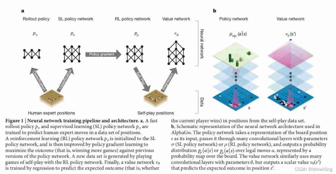
chart 1 | Neural network training pipeline and architecture .
a, Training Quick Launch Strategy p π p_π pπ And supervised learning (SL) Policy network p σ p_σ pσ To predict the movement of human experts in location data sets . Reinforcement learning (RL) Policy network p ρ p_ρ pρ Is initialized to SL Policy network , Then it is improved by strategy gradient learning , To maximize the results against the previous version of the strategic network ( Win more games ). A new dataset is created by RL Strategic network is generated by self game . Last , By returning to the training value network v θ v_θ vθ, To predict the expected results of the location in the self game data set ( That is, whether the current player wins ).
b,AlphaGo Schematic diagram of neural network architecture used in . The strategic network will place the chessboard s s s As its input , Pass it through the parameter σ σ σ(SL Policy network ) or ρ ρ ρ(RL Policy network ) Many convolutions of , And output the probability distribution p σ ( a ∣ s ) p_σ(a|s) pσ(a∣s) or p ρ ( a ∣ s ) p_ρ (a|s) pρ(a∣s) By legal movement a a a, Represented by the probability diagram on the chessboard . Value networks similarly use many parameters θ θ θ The convolution of layer , But output a scalar value v θ ( s ′ ) v_θ(s') vθ(s′) To predict the location s ′ s' s′ The expected result of .
Supervised learning of strategy network
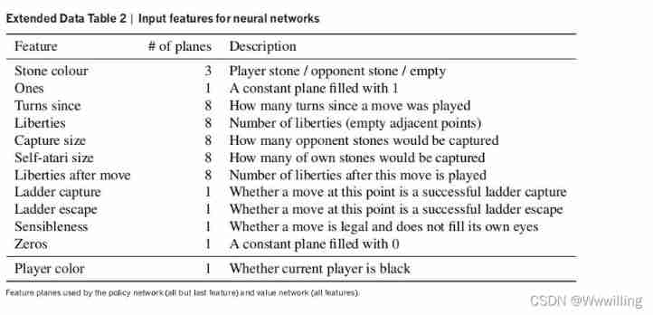
- For the first stage of the training pipeline , We build on previous work using supervised learning to predict expert actions in go games . SL Policy network p σ ( a ∣ s ) p_σ(a|s) pσ(a∣s) When the weight is σ σ σ Alternating between convolution layer and rectifier nonlinearity . the last one softmax Layer outputs all legal moves a a a Probability distribution of . Input of policy network s s s It is a simple expression of the status of the board ( See extended data sheet 2). The policy network is in the state of random sampling - The action is right ( s , a ) (s, a) (s,a) Training on , Use random gradient rise to maximize in state s s s Human movement of choice a a a The possibility of .
- We from KGS Go Server Of 3000 Ten thousand positions trained one 13 Layer policy network , We call it SL Policy network . Compared with the latest technology , The network prediction expert moves on the reserved test set , The accuracy of using all input features is 57.0%, The accuracy of using only the original chessboard position and movement history as input is 55.7% From other research groups 44.4% On the date of submission ( Extended data table 3 Complete results in ). A small increase in accuracy leads to a significant increase in performance intensity ( chart 2a); A larger network can achieve better accuracy , But the evaluation speed is slow in the search process . We also use a weight of π The linearity of small pattern characteristics softmax( See extended data sheet 4) Trained a faster but less accurate rollout Strategy p π ( a ∣ s ) p_π(a|s) pπ(a∣s); This achieved 24.2% The accuracy of , Use only 2μs To choose an action , Not the strategy of the network 3ms.

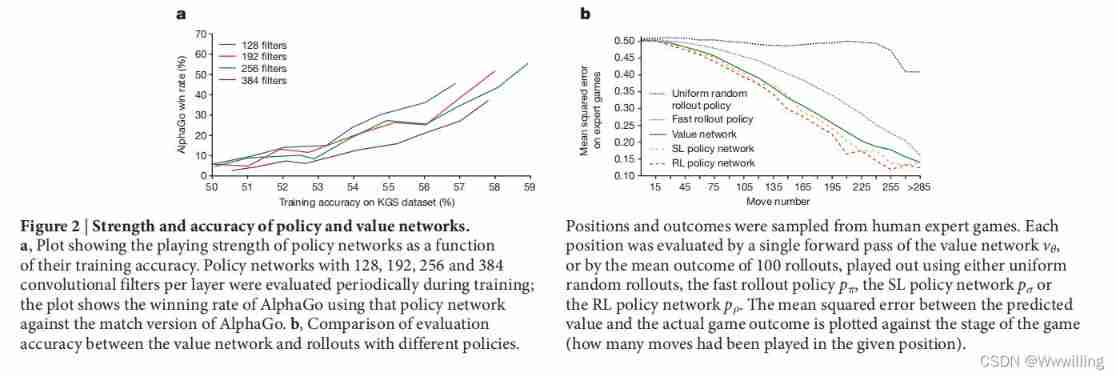
- chart 2 | Strength and accuracy of strategy and value network .
a, A graph showing the playback intensity of the strategy network as a function of its training accuracy . Evaluate each layer regularly during training 128、192、256 and 384 A strategy network of convolution filters ; This figure shows the network using this policy AlphaGo Matching version AlphaGo The winning rate .
b, Value networks and different strategies rollouts Comparison of evaluation accuracy . Locations and results are sampled from human expert Games . Every location passes through the value network v θ v_θ vθ A single forward pass of , Or through 100 Time rollout The average result of , Use uniform random rollout、 Fast rollout Strategy p π p_π pπ、SL Policy network p σ p_σ pσ or RL Policy network p ρ p_ρ pρ To assess the . The mean square error between the predicted value and the actual game result depends on the game stage ( How many steps have been taken in setting the position ) draw .
Reinforcement learning of strategy network
- The second stage of the training pipeline aims to strengthen learning through strategic gradients (RL) Improve the policy network . RL Policy network p ρ p_ρ pρ Structurally, it is similar to SL The policy is the same as the network , Its weight ρ ρ ρ Is initialized to the same value , ρ = σ ρ=σ ρ=σ. We are in the current strategic network p ρ p_ρ pρ Play the game with the randomly selected strategy network iteration before . Randomize from a group of pairs in this way to stabilize training by preventing over fitting the current strategy . We use the reward function r ( s ) r(s) r(s) For all non terminal time steps t < T t<T t<T zero . result z t = ± r ( s T ) z_t=±r(s_T) zt=±r(sT) Is in the time step t t t From the perspective of current players , The final reward at the end of the game : win +1, transport -1. Then at each time step t t t The weights are updated by a random gradient rise in the direction of maximizing the expected results .

- We assessed RL The performance of network strategy in game , Sample from the output probability distribution of each action a t ∼ p ρ ( ⋅ ∣ s t ) a_t \sim p_ρ(⋅|s_t) at∼pρ(⋅∣st). When and SL When the strategic network has a frontal confrontation ,RL Strategic networks have won 80% The above battle SL Policy network . We also target the most powerful open source Go program Pachi Tested ,Pachi Is a complex Monte Carlo search program , stay KGS Top ranked 2 Amateur segment , Perform each step 100,000 Sub simulation . Don't use search at all ,RL Strategic networks are working with Pachi Won 85% The victory of the . by comparison , The latest technology used to be based only on supervision .
- by comparison , The previous latest technology is only based on supervised learning of convolutional Networks , In the fight against Pachi Won 11% The victory of the , Against weaker programs Fuego Won 12% The victory of the .
Reinforcement learning of value network
- The final stage of the training pipeline focuses on Position Evaluation , Estimate a value function v p ( s ) v^p(s) vp(s), This function uses strategies for two players p p p To predict the location of the game being played s s s Result .
- Ideally , We want to know the perfect game v ∗ ( s ) v^*(s) v∗(s) The optimal value function under ; In practice , We use RL Policy network p ρ p_ρ pρ To estimate the value function of our strongest strategy v p ρ v^{p_ρ} vpρ. We use a weight of θ θ θ, v θ ( s ) ≈ v p ρ ( s ) ≈ v ∗ ( s ) {v_\theta }\left( s \right) \approx {v^{ {p_\rho }}}\left( s \right) \approx {v^*}\left( s \right) vθ(s)≈vpρ(s)≈v∗(s) Our value network v θ ( s ) v_θ(s) vθ(s) To approximate the value function . The neural network has a similar architecture with the strategy network , But the output is a single prediction, not a probability distribution . We pass the State - The result is right ( s , z ) (s, z) (s,z) To train the weight of the value network , Use random gradient descent to minimize the predicted value v θ ( s ) v_θ(s) vθ(s) And the corresponding results z z z Mean square error between (MSE) .

- Naive methods of predicting game results from data containing complete games can lead to over fitting . The problem is that continuous positions are strongly correlated , Only one stone is different , But the whole game shares the return goal . When in this way KGS When training on a dataset , The value network remembers the results of the game rather than generalizing to new positions , On the test set 0.37 Minimum MSE, On the training set, it is 0.19. To alleviate the problem , We have generated a new self game data set , contain 3000 Ten thousand different locations , Each location is sampled from a separate game . Every game is RL Between the strategic network and itself , Until the end of the game . The training of this data set leads to the MSE Respectively 0.226 and 0.234, Indicates that the overfitting is minimal . chart 2b It shows the location evaluation accuracy of the value network , And use fast rollout Strategy pπ Of Monte Carlo rollout comparison ; The value function is always more accurate . Yes v θ ( s ) v_θ(s) vθ(s) A single assessment of is also close to use RL Policy network p ρ p_ρ pρ Of Monte Carlo rollouts The accuracy of the , But the amount of calculation used is reduced 15,000 times .
Search with strategies and Value Networks
AlphaGo stay MCTS Algorithm ( chart 3) It combines strategy and value network , The algorithm selects actions by searching first .

chart 3 | AlphaGo Monte Carlo tree search in .
a, Each simulation has the maximum action value by selecting Q Q Q And a priori probability depending on the edge storage P P P Reward u ( P ) u(P) u(P) To traverse the tree .
b、 Leaf nodes can be extended ; The new node consists of a policy network p σ p_σ pσ Deal with it once , The output probability is stored as a priori probability of each action P P P.
c、 At the end of the simulation , Leaf nodes are evaluated in two ways : Use value networks v θ v_θ vθ; And by using the quick launch strategy p π p_π pπ Run the launch to the end of the game , And then use the function r r r Calculate the winner .
d, Update action value Q Q Q To track all evaluations in the subtree under the action r ( ⋅ ) r(·) r(⋅) and v θ ( ⋅ ) v_θ(·) vθ(⋅) Average value .Search every edge of the tree ( s , a ) (s, a) (s,a) An action value is stored Q ( s , a ) Q(s, a) Q(s,a)、 Number of visits N ( s , a ) N(s, a) N(s,a) And a priori probability P ( s , a ) P(s, a) P(s,a). The tree is traversed by simulation ( That is, drop the tree in the complete game without backup ), Start from the root state . At each time step of each simulation t t t, From the State s t s_t st Select an action in a t a_t at.
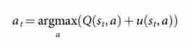
So as to maximize the action value and bonus

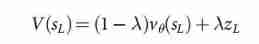
This is proportional to a priori probability , But it will decay with repeated visits to encourage exploration . When traversing in step L L L Reach leaf node s L s_L sL when , Leaf nodes can be extended . SL Policy network p σ p_σ pσ Only handle leaf positions s L s_L sL once . Output probability as every legal action a a a The prior probability of P P P Storage , P ( s ∣ a ) = P σ ( a ∣ s ) P(s|a)= P_σ(a|s) P(s∣a)=Pσ(a∣s) . Leaf nodes are evaluated in two distinct ways : First , Through value networks v θ ( s L ) v_θ(s_L) vθ(sL); secondly , According to the use of quick launch strategy p π p_π pπ The random results of z L z_L zL, Until the terminal step T T T until ; Using mixed parameters λ λ λ Combine these assessments into leaf assessments V ( s L ) V(s_L) V(sL)
At the end of the simulation , Update the action value and access count of all traversal edges . Each edge accumulates the access count and average evaluation of all simulations through that edge

among s L i {s_L}^i sLi It's No i i i Leaf nodes of secondary simulation , 1 ( s , a , i ) 1(s, a, i) 1(s,a,i) Said in the first i i i Whether the edges were traversed during the second simulation ( s , a ) (s, a) (s,a). When the search is complete , The algorithm selects the most visited mobile from the root location .
It is worth noting that ,SL Policy network p σ p_σ pσ stay AlphaGo In the performance than stronger RL Policy network p ρ p_ρ pρ Better , This is probably because human beings have chosen a series of promising ways , and RL Optimized the single best walking method . However , From stronger RL Value function derived from policy network v θ ( s ) ≈ v p ρ ( s ) {v_\theta }\left( s \right) \approx {v^{ {p_\rho }}}\left( s \right) vθ(s)≈vpρ(s) stay AlphaGo Zhongbi from SL Value function derived from policy network v θ ( s ) ≈ v p σ ( s ) {v_\theta }\left( s \right) \approx {v^{ {p_\sigma }}}\left( s \right) vθ(s)≈vpσ(s) Perform better .
Evaluation strategies and value networks require several orders of magnitude more computation than traditional search heuristics . In order to effectively MCTS Combined with deep neural networks ,AlphaGo Use asynchronous multithreading to search in CPU Perform simulation on , And in GPU Parallel computing strategy and value network . AlphaGo The final version of uses 40 Search threads 、48 individual CPU and 8 individual GPU. We also implemented a distributed version AlphaGo, It uses several machines 、40 Search threads 、1,202 individual CPU and 176 individual GPU. The method section provides asynchronous and distributed MCTS Full details of .
assessment AlphaGo Chess power
- To evaluate AlphaGo, We are AlphaGo An internal game was held between the variant of go and several other go programs , These include the strongest business processes Crazy Stone and Zen, And the strongest open source program Pachi and Fuego. All these programs are based on high-performance MCTS Algorithm . Besides , We also include open source programs GnuGo, This is a use of MCTS The most advanced search method before Go Program . All programs are allowed to have 5 Second count time .
- The result of the championship ( See the picture 4a) indicate , stand-alone AlphaGo It is much stronger than any previous Go program , In connection with other go programs 495 Won the game 494 site (99.8%). To give AlphaGo Provide greater challenges , We also made four concessions ( That is, the opponent is free to go ) The match of ; AlphaGo Respectively by 77%、86% and 99% Our winning rate defeated Crazy Stone、Zen and Pachi. AlphaGo The distributed version of is significantly more powerful , For single machine AlphaGo The winning rate of the competition is 77%, The winning rate against other programs is 100%.
- We also evaluated the use of value networks only ( λ = 0 ) (λ = 0) (λ=0) Or use only rollouts ( λ = 1 ) (λ = 1) (λ=1) Evaluate the location AlphaGo variant ( See the picture 4b). Even if it is not launched ,AlphaGo It also exceeds the performance of all other go programs , This shows that the value network provides a feasible alternative to Monte Carlo evaluation in go . However , Mixed assessment (λ=0.5) Perform best , Winning rate against other variants ≥95%. This shows that the two location evaluation mechanisms are complementary : The value network is close to strong but unrealistically slow pρ The result of the game played , and rollouts Can accurately score and evaluate weak but fast rollout Strategy pπ The result of the game played . chart 5 Shows AlphaGo Evaluation of real game location .

- chart 4 | AlphaGo Competition evaluation .
a, Game results between different Go programs ( See extended data sheet 6-11). Each program uses about 5 Second count time . In order to AlphaGo Provide greater challenges , Some procedures ( Pale upper bar ) Be given four pieces of chess ( That is, the free step at the beginning of each game ) Against all opponents . The evaluation of the procedure adopts Elo gauge 37:230 The difference of points corresponds to 79% The probability of winning , Roughly corresponds to KGS38 An amateur position advantage on ; It also shows the approximate correspondence with the human level , The horizontal line shows what the program gets online KGS Grade . The competition with human European champion fan Hui is also included ; These games use longer time control . Shows 95% The confidence interval of .
b, AlphaGo On a single machine , Performance of different component combinations . Only use the version of the policy network without performing any search .
c, Use asynchronous search ( The light blue ) Or distributed search ( Navy Blue ), stay AlphaGo Search threads and GPU Conduct MCTS Research on scalability of , Every step 2 second .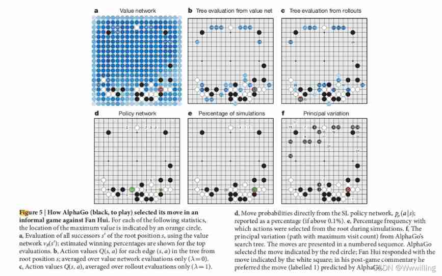
- chart 5 | AlphaGo( Black chess , Playing chess ) How to choose chess moves in the informal game with fan Hui . For each of the following statistics , The position of the maximum value is indicated by an orange circle .
a, Use value networks v θ ( s ′ ) v_θ(s') vθ(s′) Evaluate root location s s s All the successors of s ′ s' s′; Show the estimated winning percentage of the highest rating .
b, From the root of the tree s s s Start each side ( s , a ) (s, a) (s,a) Action value of Q ( s , a ) Q(s, a) Q(s,a); Only average the value network evaluation ( λ = 0 ) (λ=0) (λ=0).
c, Action value Q ( s , a ) Q(s, a) Q(s,a), Only in rollout Average the evaluation ( λ = 1 ) (λ=1) (λ=1).
d, Directly from SL Strategic network mobility probability , p σ ( a ∣ s ) p_σ(a|s) pσ(a∣s); Report as a percentage ( If it is higher than 0.1%).
e, Select the percentage frequency of actions from the root during simulation .
f, come from AlphaGo The main variants of the search tree ( The path with the maximum number of accesses ). These actions are presented in numbered order . AlphaGo Choose the walking method shown in the red circle ; Fan Hui responded with the action shown by the white square ; In his post game comments , He likes it better AlphaGo The way of prediction ( Marked as 1). - Last , We will distribute the version AlphaGo And professional 2 A chess player 、2013、2014 and 2015 Fan Hui, the champion of the European Go Championship in, made a comparison . 2015 year 10 month 5 solstice 9 Japan ,AlphaGo A formal five game match with fan Hui . AlphaGo With 5 Than 0 Win the game ( chart 6 And extended data table 1). This is the first time that a computer Go program has defeated a human professional player in a complete go game without obstacles —— Previously, it was believed that this feat would take at least ten years to achieve .

- chart 6 | AlphaGo Competition with European champion fan Hui .
The movements are displayed in numbered order corresponding to the order in which they are played . Repeated movements at the same intersection are displayed in pairs below the chessboard . The first movement number in each pair indicates the time of repeated movement , At the intersection identified by the second mobile number ( See Supplementary information ).
Discuss
- In this work , We developed a go program based on the combination of deep neural network and tree search , It works at the level of the strongest human player , Thus, the artificial intelligence “ Major challenges ” One of . For the first time, we have developed an effective go move selection and position evaluation function , Based on deep neural network , These networks are trained through a novel combination of supervised learning and reinforcement learning . We introduce a new search algorithm , The algorithm successfully combines neural network evaluation with Monte Carlo rollouts Combination . Our program AlphaGo Large scale integration of these components in a high-performance tree search engine .
- AlphaGo The match with fan Hui , Thousands of times less than the chess game between dark blue and Kasparov ; Compensate by selecting these positions more intelligently , Use policy network , And use value networks to evaluate them more accurately —— A method that may be closer to the human way of playing . Besides , Although dark blue relies on handmade evaluation functions , but AlphaGo The neural network of is trained directly from game playing through general supervision and reinforcement learning methods .
- Go is in many ways a model of the difficulties faced by AI : Challenging decision-making tasks 、 Difficult search space and such a complex optimal solution , So that it seems infeasible to use strategy or value function to approach directly . Previous major breakthroughs in computer go ,MCTS The introduction of , It has led to corresponding progress in many other fields ; for example , General games 、 Classic planning 、 Partial observation planning 、 Scheduling and constraints meet . By combining tree search with strategy and value network ,AlphaGo Finally reached a professional level in go , It provides hope that human level performance can now be achieved in other seemingly intractable AI fields .
Method
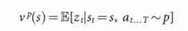
- Question setting . Many complete information games , Like chess 、 Checkers 、 Othello 、 Backgammon and go , It can be defined as alternating Markov game . In these games , There is a state space S S S( The status includes the instructions that the current player wants to play ); An action space A ( s ) A(s) A(s) Defines any given state s ∈ S s \in S s∈S Legal actions in ; State transition functions f ( s , a , ξ ) f(s, a, ξ) f(s,a,ξ) Defined in the state s s s Choose the action a a a And random input ξ ξ ξ( For example, dice ) Subsequent state after ; The last reward function r i ( s ) r^i(s) ri(s) Describes the player i i i In state s s s Rewards received in . We limit our attention to the two person zero sum game , r 1 ( s ) = − r 2 ( s ) = r ( s ) r^1(s)=−r^2(s)=r(s) r1(s)=−r2(s)=r(s), With deterministic state transition , f ( s , a , ξ ) = f ( s , a ) f(s, a, ξ)=f(s, a) f(s,a,ξ)=f(s,a), Except in the terminal time step T T T outside , Zero reward . The result of the game z t = ± r ( s T ) z_t=±r(s_T) zt=±r(sT) It's in the time step t t t From the perspective of the current player, the terminal reward at the end of the game . Strategy p ( a ∣ s ) p(a|s) p(a∣s) It's a legal act a ∈ A ( s ) a \in A(s) a∈A(s) Probability distribution of . If according to the strategy p p p Choose all the actions of the two participants , Then the value function is the expected result , namely v p ( s ) = E [ z t ∣ s t = s , a t . . . T ∼ p ] v^p(s)=E[z_t|s_t=s,a_t...T \sim p] vp(s)=E[zt∣st=s,at...T∼p] . Zero sum games have a unique optimal value function v ∗ ( s ) v^*(s) v∗(s), It determines the perfect post game state of two players s s s Result ,

- Previous work . The optimal value function can be obtained by minimax( Or equivalent negamax) Search recursive calculation . Most games are minimal for detailed imax It's too big for tree search ; contrary , By using an approximation function v ( s ) ≈ v ∗ ( s ) v(s)≈v^*(s) v(s)≈v∗(s) Instead of terminal rewards to cut the game . Use alpha-beta pruning Depth first minimax search in chess 、 He achieved superhuman performance in checkers and black and white , But the effect is not good in go .
- Reinforcement learning can directly learn the approximate optimal value function from self game . Most previous work has focused on features ϕ ( s ) ϕ(s) ϕ(s) And weight θ θ θ The linear combination of v θ ( s ) = ϕ ( s ) ⋅ θ v_θ(s)=ϕ(s)· θ vθ(s)=ϕ(s)⋅θ. At chess 、 Checkers and go use time difference to learn training weights ; Or use linear regression in black and white and scrabble . TDOA learning is also used to train neural networks to approximate the optimal value function , Achieve superhuman performance in backgammon ; The convolution network is used to realize weak kyu Class performance .
- Another method of minimax search is Monte Carlo tree search (MCTS), It estimates the optimal value of internal nodes by double approximation , V n ( s ) ≈ v p n ( s ) ≈ v ∗ ( s ) {V^n}\left( s \right) \approx {v^{ {p^n}}}\left( s \right) \approx {v^*}\left( s \right) Vn(s)≈vpn(s)≈v∗(s) . First approximation V n ( s ) ≈ v p n ( s ) {V^n}\left( s \right) \approx {v^{ {p^n}}}\left( s \right) Vn(s)≈vpn(s) Use n n n Monte Carlo simulation is used to estimate the simulation strategy P n P_n Pn The value function of . The second approximation v p n ( s ) ≈ v ∗ ( s ) {v^{ {p^n}}}\left( s \right) \approx {v^*}\left( s \right) vpn(s)≈v∗(s) Use simulation strategy P n P_n Pn Instead of minimax optimal action . The simulation strategy is based on the search control function ( Q n ( s , a ) + u ( s , a ) ) \left( { {Q^n}\left( {s,a} \right) + u\left( {s,a} \right)} \right) (Qn(s,a)+u(s,a)) Choose action , for example UCT, This function selects child nodes with higher action values , Q n ( s , a ) = − V n ( f ( s , a ) ) {Q^n}\left( {s,a} \right) = - {V^n}\left( {f\left( {s,a} \right)} \right) Qn(s,a)=−Vn(f(s,a)), Plus rewards u ( s , a ) u(s, a) u(s,a) Encourage exploration ; Or in the state s s s Without a search tree , It starts with a quick launch strategy p π ( a ∣ s ) p_π(a|s) pπ(a∣s) Sampling action in . As more simulations are performed and the search tree becomes deeper , Simulation strategies become more and more accurate statistics . In extreme cases , Both approximations become accurate and MCTS( for example , Use UCT) Converge to the optimal value function lim n → ∞ V n ( s ) = lim n → ∞ v p n ( s ) = v ∗ ( s ) {\lim _{n \to \infty }}{V^n}\left( s \right) = {\lim _{n \to \infty }}{v^{ {p^n}}}\left( s \right) = {v^*}\left( s \right) limn→∞Vn(s)=limn→∞vpn(s)=v∗(s). The most powerful Go program at present is based on MCTS.
- MCTS It has been previously combined with a strategy for reducing the beam of the search tree to high probability movement ; Or shift the bonus items to high probability . MCTS It also combines a value function , Used to initialize the action value in the newly extended node , Or combine Monte Carlo evaluation with minimax evaluation . by comparison ,AlphaGo The use of the value function is based on the truncated Monte Carlo search algorithm , The algorithm terminates before the end of the game , And use value function instead of terminal reward . AlphaGo The location assessment is mixed with the complete rollout And truncated rollout, In some ways, it is similar to the well-known time difference learning algorithm TD(λ). AlphaGo It is also different from the previous work , It uses a slower but more powerful strategy and value function representation ; The evaluation depth neural network is several orders of magnitude slower than the linear representation , Therefore, it must occur asynchronously .
- MCTS The performance of depends largely on the quality of the launch strategy . Previous work focused on learning through supervision 、 Reinforcement learning 、 Simulate balance or online adaptation to make patterns by hand or learn promotion strategies ; However , as everyone knows , be based on rollout The location assessment of is often inaccurate . AlphaGo It's relatively simple to use rollout, Instead, use the value network to solve the challenging problem of location evaluation more directly .
- search algorithm . In order to effectively integrate large-scale neural networks into AlphaGo in , We implemented asynchronous policies and values MCTS Algorithm (APV-MCTS). Search every node in the tree s s s Include all legal actions a ∈ A ( s ) a \in A(s) a∈A(s) The edge of ( s , a ) (s, a) (s,a) . Each edge stores a set of Statistics ,

- among P ( s , a ) P(s, a) P(s,a) It's a priori probability , W v ( s , a ) W_v(s, a) Wv(s,a) and W r ( s , a ) W_r(s, a) Wr(s,a) Is the Monte Carlo estimation of the total action value , stay N v ( s , a ) N_v(s, a) Nv(s,a) and N r ( s , a ) N_r(s, a) Nr(s,a) Accumulate on ) They are leaf evaluation and rollout Reward , Q ( s , a ) Q(s, a) Q(s,a) Is the combined average action value of this side . Multiple simulations are executed in parallel on separate search threads . APV-MCTS The algorithm is shown in Figure 3.
- choice ( chart 3a). The first of each simulation in-tree The stage starts at the root of the search tree , When the simulation is in time step L L L End when reaching the leaf node . At each time step t < L t<L t<L in , Select an action based on the statistics in the search tree , a t = arg max a ( Q ( s t , a ) + u ( s t , a ) ) {a_t} = \arg {\max _a}\left( {Q\left( { {s_t},a} \right) + u\left( { {s_t},a} \right)} \right) at=argmaxa(Q(st,a)+u(st,a)) Use PUCT Variants of the algorithm p, among cpuct Is a constant that determines the level of exploration ; This search control strategy initially preferred actions with high a priori probability and low access times , But I gradually like actions with high action value . In each of these time steps , t < L t<L t<L, Choose an action based on statistics In the search tree in ,t Use PUCT Variants of the algorithm u ( s , a ) = c p u c t P ( s , a ) ∑ b N r ( s , b ) 1 + N r ( s , b ) u\left( {s,a} \right) = {c_{puct}}P\left( {s,a} \right)\frac{ {\sqrt {\sum\nolimits_b { {N_r}\left( {s,b} \right)} } }}{ {1 + {N_r}\left( {s,b} \right)}} u(s,a)=cpuctP(s,a)1+Nr(s,b)∑bNr(s,b) , among c p u c t c_{puct} cpuct Is a constant that determines the level of exploration ; This search control strategy initially preferred actions with high a priori probability and low access times , But I gradually like actions with high action value .
- assessment ( chart 3c). The value network will be leaf position s L s_L sL Added to the queue for evaluation v θ ( s L ) v_θ(s_L) vθ(sL), Unless it has been evaluated before . The second stage of each simulation is derived from leaf nodes s L s_L sL Start , Continue until the end of the game . In each of these time steps , t ≥ L t≥L t≥L, Both players choose actions according to the launch strategy , a t ∼ p π ( ⋅ ∣ s t ) a_t \sim p_π(⋅|s_t) at∼pπ(⋅∣st). When the game reaches its final state , result z t = ± r ( s T ) z_t= ± r(s_T) zt=±r(sT) Calculated from the final score .
- Backup ( chart 3d). In each of the simulations in-tree step t ≤ L t≤L t≤L It's about , to update rollout statistics , It's like it's lost n v l n_{vl} nvl game , N r ( s t , a t ) ← N r ( s t , a t ) + n v l N_r(s_t, a_t)←N_r(s_t, a_t)+n_{vl} Nr(st,at)←Nr(st,at)+nvl; W r ( s t , a t ) ← W r ( s t , a t ) − n v l W_r(s_t, a_t)←W_r(s_t, a_t) -n_{vl} Wr(st,at)←Wr(st,at)−nvl; This virtual loss prevents other threads from exploring the same changes at the same time . At the end of the simulation , At every step t ≤ L t≤L t≤L Update in the reverse transfer of rollout Statistics , Use the results N r ( s t , a t ) ← N r ( s t , a t ) − n v l + 1 N_r(s_t, a_t)←N_r(s_t, a_t) -n_{vl}+1 Nr(st,at)←Nr(st,at)−nvl+1 Replace virtual losses ; W r ( s t , a t ) ← W r ( s t , a t ) + n v l + z t W_r(s_t, a_t)←W_r(s_t, a_t)+n_{vl}+z_t Wr(st,at)←Wr(st,at)+nvl+zt. Asynchronously , When the leaf position s L s_L sL When the assessment of is completed , A separate reverse transfer will be initiated . The output of the value network v θ ( s L ) v_θ(s_L) vθ(sL) Used to update value statistics in the second back propagation , Through each step t ≤ L t ≤ L t≤L, N v ( s t , a t ) ← N v ( s t , a t ) + 1 N_v(s_t, a_t)←N_v(s_t, a_t)+1 Nv(st,at)←Nv(st,at)+1, W v ( s t , a t ) ← W v ( s t , a t ) + v θ ( s L ) W_v(s_t, a_t) ←W_v(s_t, a_t)+v_θ(s_L) Wv(st,at)←Wv(st,at)+vθ(sL). The overall assessment of each state action is Monte Carlo Estimated value λ λ λ Weighted average of , It combines value networks with rollout Evaluation and weighting parameters λ λ λ Mix it up . All updates are performed without locks .
- Expand ( chart 3b). When the number of visits exceeds the threshold N r ( s , a ) > n t h r N_r(s, a)>n_{thr} Nr(s,a)>nthr when , Follow up status s ′ = f ( s , a ) s'=f(s, a) s′=f(s,a) Add to the search tree . The new node is initialized to { N ( s ′ , a ) = N r ( s ′ , a ) = 0 , W ( s ′ , a ) = W r ( s ′ , a ) = 0 , P ( s ′ , a ) = p σ ( a ∣ s ′ ) } \{ N(s', a)=N_r(s', a)=0, W(s', a)=W_r(s', a)=0, P(s',a) =p_σ(a|s') \} { N(s′,a)=Nr(s′,a)=0,W(s′,a)=Wr(s′,a)=0,P(s′,a)=pσ(a∣s′)}, Use tree strategy p τ ( a ∣ s ′ ) p_τ(a|s') pτ(a∣s′)( Be similar to rollout Strategy , But it has more functions , See extended data table 4) Provide placeholder prior probability for action selection . Location s ′ s' s′ Also inserted into a queue , Asynchronous for Policy Networks GPU assessment . A priori probability is determined by SL Policy network p σ β ( ⋅ ∣ s ′ ) {p_σ}^β(⋅|s′) pσβ(⋅∣s′) Calculation ,softmax The temperature is set to β β β; These replace placeholder prior probabilities with atomic updates $P( s′,a) ← {p_σ}^β(a|s′) . threshold n t h r n_{thr} nthr It's dynamically adjusted , To ensure that the rate at which locations are added to the policy queue is the same as GPU Evaluate the speed of the policy network to match . Location is used by strategic networks and Value Networks mini-batch The size is 1 To assess the , To minimize end-to-end evaluation time .
- We also implemented distributed APV-MCTS Algorithm . The architecture consists of a single host that performs a master search 、 Perform multiple remote jobs for asynchronous deployment CPU And multiple remote jobs that perform asynchronous policy and value network assessments GPU form . The entire search tree is stored in master On , It only performs each simulated in-tree Stage . Leaf position and execution simulation of the work of the launch phase CPU And work GPU communicate , The latter calculates network characteristics and evaluates strategies and value networks . The prior probability of the policy network is returned to the master node , There they replace the placeholder prior probability of the new extension node . come from rollout The reward and value network output of are returned to master, And back up the original search path .
- At the end of the search ,AlphaGo Select the action with the most visits ; Compared with maximizing the action value , This is not very sensitive to outliers . The search tree is reused in subsequent time steps : The child node corresponding to the playback action becomes the new root node ; The subtree below this subtree and all its statistical data are preserved , And the rest of the tree is discarded . AlphaGo The game version of continues to search while the opponent is moving . If the operation of maximizing access times is inconsistent with the operation of maximizing operation value , Then expand the search . Time control is designed to use most of the time in the middle of the game . When AlphaGo The overall assessment of is lower than estimated 10% The probability of winning the game , namely m a x a Q ( s , a ) < − 0.8 max_aQ(s,a)<-0.8 maxaQ(s,a)<−0.8 when ,AlphaGo Will resign .
- AlphaGo Not using all the moves or quick action value estimation methods used in most Monte Carlo Go programs ; When using policy networks as prior knowledge , These biased heuristics don't seem to bring any additional benefits . Besides ,AlphaGo Do not use progressive widening 、 dynamic komi Or start . AlphaGo The parameters used in fan Hui's competition are listed in the extended data table 5 in .

- Rollout policy. rollout Strategy p π ( a ∣ s ) p_π(a|s) pπ(a∣s) It is based on fast 、 Incremental calculation 、 Linearity based on the characteristics of local patterns softmax Strategy , Including the resulting state s s s The previous one moves around “ Respond to ” Patterns and surrounding “ No response ” Mode candidate in state s s s In the mobile a a a. Each unresponsive pattern is a binary feature , Match with a a a Centered on specific 3×3 Pattern , By the color of each adjacent intersection ( black 、 white 、 empty ) And free counting (1、2、≥3) Definition . Each response pattern is a binary feature , With the previous move as the center 12 Dot diamond pattern 21 The color in matches the free count . Besides , A small number of handmade local feature codes common sense go rules ( See extended data sheet 4). Similar to policy networks ,rollout Weight of strategy π π π It's from Tygem Human games on the server 800 Training in 10000 positions , To maximize log likelihood through random gradient descent . On the empty board , Every CPU Threads execute about per second 1,000 Sub simulation .
- Our launch strategy p π ( a ∣ s ) p_π(a|s) pπ(a∣s) It contains less manual knowledge than the most advanced Go program . contrary , We make use of MCTS Medium and higher quality action choices , This is notified by the search tree and Policy Network . We introduced a new technology , You can cache all movements in the search tree , Then play a similar move during the launch ; “ The last good reply ” Heuristic generalization . At every step of tree traversal , The most likely actions are inserted into a hash table , And around the previous move and the current move 3×3 Schema context ( Color 、 Degrees of freedom and stone counting ). stay rollout Every step of , The schema context will match the hash table ; If a match is found , Then the storage is moved with a high probability .
- symmetry . In previous work , By using rotation and reflection invariant filters in the convolution layer Go The symmetry of . Although this may be effective in small neural networks , But it will actually damage the performance of large networks , Because it will prevent the intermediate filter from recognizing specific asymmetric patterns . contrary , We use a dihedral group of eight reflections and rotations d 1 ( s ) , … , d 8 ( s ) d_1(s), …, d_8(s) d1(s),…,d8(s) Dynamically transform each position s s s Use symmetry at runtime . In explicit symmetric integration , all 8 Small batches of locations are transferred to the strategy network or value network and calculated in parallel . For Value Networks , The output values are simply averaged .

- For policy networks , The output probability plane is rotated / Reflect back to the original direction , And averaged together to provide integrated forecasts σ σ σ ; This method is used in our original network evaluation ( See extended data sheet 3). contrary ,APV-MCTS Use implicit symmetric integration , Select a single rotation randomly for each evaluation / Reflection j ∈ [ 1 , 8 ] j \in [1, 8] j∈[1,8]. We only calculate one assessment in this direction ; In each simulation , We go through v θ ( d j ( s L ) ) v_θ(d_j(s_L)) vθ(dj(sL)) Calculate leaf nodes s L s_L sL Value , And allow the search process to average these assessments . Similarly , We choose the rotation for a single random / Reflective computing strategy network

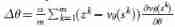
- Policy network : classification . Our training strategy network p σ p_σ pσ Based on KGS Expert actions in the dataset classify locations . The dataset contains KGS 6 to 9 Human players play 160,000 In a game 2940 10000 locations ; 35.4% Our game is a handicap game . Data sets are divided into test sets ( The first onemillion positions ) Training set ( rest 2840 10000 locations ). Passing is excluded from the data set . Each position is described by the original chessboard s s s And the movement of human choice a a a form . We expanded the data set to include all eight reflections and rotations for each location . Symmetry enhancement and input features are pre calculated for each position . For each training step , We start from enhanced KGS Randomly selected in the data set m m m A small batch of samples , { s k , a k } k = 1 m \left\{ { {s^k},{a^k}} \right\}_{k = 1}^m { sk,ak}k=1m Asynchronous random gradient descent update is applied to maximize the log likelihood of the action , Δ σ = a m ∑ k = 1 m ∂ log p σ ( a k ∣ s k ) ∂ σ \Delta \sigma = \frac{a}{m}\sum\nolimits_{k = 1}^m {\frac{ {\partial \log {p_\sigma }\left( { {a^k}|{s^k}} \right)}}{ {\partial \sigma }}} Δσ=ma∑k=1m∂σ∂logpσ(ak∣sk). step α α α Initialize to 0.003, Every time 8000 Halve 10000 training steps , There is no momentum term , The small batch size is m = 16 m=16 m=16. Use DistBelief stay 50 individual GPU Apply updates asynchronously on ; exceed 100 The gradient of step is discarded . 3.4 100 million training steps need about 3 weeks .
- Policy network : Reinforcement learning . We further train the strategy network through strategy gradient reinforcement learning . Each iteration involves small batches running in parallel n n n A game , In the strategy network currently being trained p ρ p_ρ pρ And use parameters from previous iterations ρ − ρ^- ρ− The opponent p ρ − {p_ρ}^− pρ− Between , Random sampling from the pool to increase the stability of training . The weight is initialized to ρ = ρ − = σ ρ=ρ^− =σ ρ=ρ−=σ. Every time 500 Sub iteration , We will use the current parameter ρ ρ ρ Add to the opponent pool . Every game in a small batch i i i Proceed to step T i T_i Ti End , Then score from the perspective of each player to determine the result z t i = ± r ( s T i ) z_t^i = \pm r\left( { {s_{ {T^i}}}} \right) zti=±r(sTi). Then replay the game to determine the strategy gradient update , Δ ρ = a n ∑ i = 1 n ∑ t = 1 T i ∂ log p ρ ( a t i ∣ s t i ) ∂ ρ ( z t i − v ( s t i ) ) \Delta \rho = \frac{a}{n}\sum\nolimits_{i = 1}^n {\sum\nolimits_{t = 1}^{ {T^i}} {\frac{ {\partial \log {p_\rho }\left( {a_t^i|{s_t}^i} \right)}}{ {\partial \rho }}} } \left( {z_t^i - v\left( {s_t^i} \right)} \right) Δρ=na∑i=1n∑t=1Ti∂ρ∂logpρ(ati∣sti)(zti−v(sti)), Use REINFORCE Algorithm And baseline v ( s t i ) {v\left( {s_t^i} \right)} v(sti) For variance reduction . When I first passed the training channel , The baseline is set to zero ; In the second pass , We use value networks v θ ( s ) v_θ(s) vθ(s) As a baseline ; This provides a small performance improvement . In this way, the strategy network has been trained for a day , Use 50 individual GPU, Yes 128 A game 10,000 A small batch of training .
- Value network : Return to . We trained a value network v θ ( s ) ≈ v p ρ ( s ) v_θ(s) \approx v^{p_ρ}(s) vθ(s)≈vpρ(s) To approximate RL Policy network p ρ p_ρ pρ The value function of . In order to avoid over fitting strongly related positions in the game , We constructed a new dataset of unrelated self game positions . This dataset contains more than 3000 10000 locations , Each position comes from a unique self game . Every game is sampled by random time steps U ∼ u n i f { 1 , 450 } U \sim unif \{1, 450 \} U∼unif{ 1,450} And from SL Before sampling in the policy network t = 1 , … U − 1 t=1,… U−1 t=1,…U−1 Move , a t ∼ p σ ( ⋅ ∣ s t ) a_t \sim p_σ(·|s_t) at∼pσ(⋅∣st) To generate in three stages ; Then sample a move randomly and evenly from the available moves , a U ∼ u n i f { 1 , 361 } a_U \sim unif \{1, 361 \} aU∼unif{ 1,361}( Repeat until a U a_U aU legal ); And then from RL Policy network a t ∼ p ρ ( ⋅ ∣ s t ) a_t \sim p_ρ(·|s_t) at∼pρ(⋅∣st) Sample the remaining moving sequence , Until the end of the game , t = U + 1 , … T t=U+1, … T t=U+1,…T. Last , Rate the game to determine the result z t = ± r ( s T ) z_t=±r(s_T) zt=±r(sT). Only one training example is added to the dataset of each game ( s U + 1 , z U + 1 ) (s_{U+1}, z_{U+1}) (sU+1,zU+1). This data provides an unbiased sample of the value function .

- In the first two stages of generation , We sample from a noisy distribution , To increase the diversity of data sets . Training methods and SL Strategy network training is the same , The difference is that the parameter update is based on the mean square error between the predicted value and the observed reward ,
- Value network usage 50 individual GPU Yes 32 Location 5000 Ten thousand small batches have been trained for a week .
- Strategy / The function of value network . Each position s s s Be pretreated into a group 19×19 The characteristic plane of . The features we use come directly from the original representation of the rules of the game , Indicates the state of each intersection of the go board : The color of the pieces 、 freedom ( Adjacent empty points of chess chain )、 Capture 、 Legitimacy 、 The number of rounds since playing chess , and ( Only applicable to value networks ) Current color to play . Besides , We use a simple tactical feature to calculate the results of ladder search . All features are calculated relative to the current color to be played ; for example , The stone color of each intersection is represented by the player or opponent , Not black or white . Each integer eigenvalue is divided into multiple 19×19 Binary value of plane (one-hot encoding). for example , A separate binary feature plane is used to indicate whether the intersection has 1 individual liberties free 、2 A freedom 、……、≥8 A freedom . The complete feature plane set is listed in the extended data table 2 in .
- Neural network architecture . The input of policy network is made by 48 Composed of characteristic planes 19×19×48 Image stack . The first hidden layer zero fills the input with 23×23 Image , And then k k k Kernel size is 5×5 The filter of is convoluted with the input image , The stride is 1, And apply rectifier nonlinearity . Subsequent hidden layers 2 To 12 Each of them fills its previous hidden layer zero into a 21×21 In the image of , And then k k k Kernel size is 3×3 Filter and step size 1 Convolution , Follow the nonlinear rectifier again . Finally, the kernel size is 1×1 Of 1 Filters and steps 1 Convolution , Each position has a different deviation , And Application softmax function . AlphaGo The competition version of uses k = 192 k=192 k=192 A filter ; chart 2b And extended data table 3 It also shows the use k = 128、256 and 384 Training results of filters .
- The input of value network is also a 19×19×48 Image stack , There is also an additional binary feature plane to describe the current color to be played . Hidden layer 2 To 11 Same as policy network , Hidden layer 12 Is an additional convolution layer , Hidden layer 13 Convolution 1 Kernel size is 1×1 Filter for , The stride is 1, Hidden layer 14 Is a fully connected linear layer , Yes 256 Rectifier units . The output layer has a single tanh The fully connected linear layer of the unit .
- assessment . We conduct internal tournaments and measure the performance of each program Elo Grade to evaluate the relative strength of computer Go programs . We use logical functions

- Estimation procedure a Defeat the program b Probability , And pass BayesElo The program uses standard constants c e l o = 1 / 400 c_{elo}=1/400 celo=1/400 Calculated Bayesian logistic regression estimation score e ( ⋅ ) e(·) e(⋅). The scale is based on fan Hui, a professional go player BayesElo score ( The date of submission is 2,908). All programs can receive up to 5 Second count time ; The competition uses Chinese rules to score , Komi Wei 7.5 branch ( Bonus points to compensate for the second place in white chess ). We also played let AlphaGo Playing white chess with the existing go program ; For these games , We use a non-standard subsystem , Among them, Komi , But the black extra stone is given on the usual parting point . Use these rules , K K K The making points of a chess piece is equivalent to giving black chess K − 1 K-1 K−1 Step free step , Instead of using standard none Komi Let's be regular K − 1 / 2 K-1/2 K−1/2 A free step . We use these rules because AlphaGo The value network is specially trained for use 7.5 Of komi.
- Except for distributed AlphaGo outside , Each computer Go program is executed on its own stand-alone , With the same specifications , Use the latest available version and the best hardware configuration supported by the program ( See extended data sheet 6). In the figure 4 in , The approximate ranking of computer programs is based on the highest achieved by the program KGS ranking ; however ,KGS The version may be different from the public version .
- The game against fan Hui will be arbitrated by an impartial referee . 5 A formal match and 5 An informal match with 7.5 komi、 There is no upper limit and Chinese rules . AlphaGo Respectively by 5-0 and 3-2 Won these games ( chart 6 And extended data table 1). The time control of the official competition is 1 Hours plus three 30 Second race time . The time control of informal games is three 30 second byoyomi. Before the game, fan Hui chose time control and competition conditions ; It is also agreed that the overall result of the competition will be completely determined by the official competition . In order to roughly evaluate fan Hui's relative rating of computer Go programs , We add the results of all ten games to our internal game results , Ignoring the difference in time control .
边栏推荐
- VR/AR 的产业发展与技术实现
- Matlab r2021b installing libsvm
- 咋吃都不胖的朋友,Nature告诉你原因:是基因突变了
- The function of carbon brush slip ring in generator
- JVM memory and garbage collection-3-object instantiation and memory layout
- Cross modal semantic association alignment retrieval - image text matching
- VIM string substitution
- The method of using thread in PowerBuilder
- CorelDRAW2022下载安装电脑系统要求技术规格
- 牛熊周期与加密的未来如何演变?看看红杉资本怎么说
猜你喜欢
软件测试笔试题你会吗?

Nanny level tutorial: Azkaban executes jar package (with test samples and results)
leetcode 866. Prime Palindrome | 866. 回文素数
![[reinforcement learning medical] deep reinforcement learning for clinical decision support: a brief overview](/img/45/5f14454267318bb404732c2df5e03c.jpg)
[reinforcement learning medical] deep reinforcement learning for clinical decision support: a brief overview
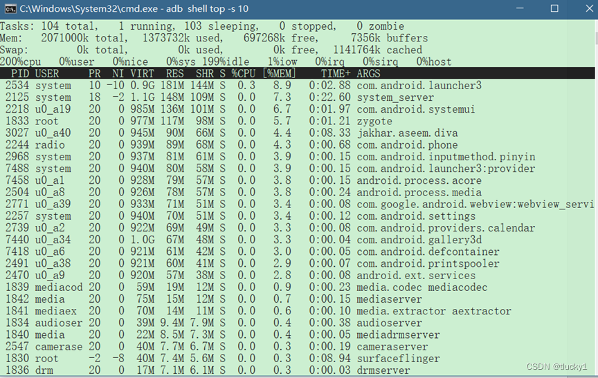
Introduction to ADB tools
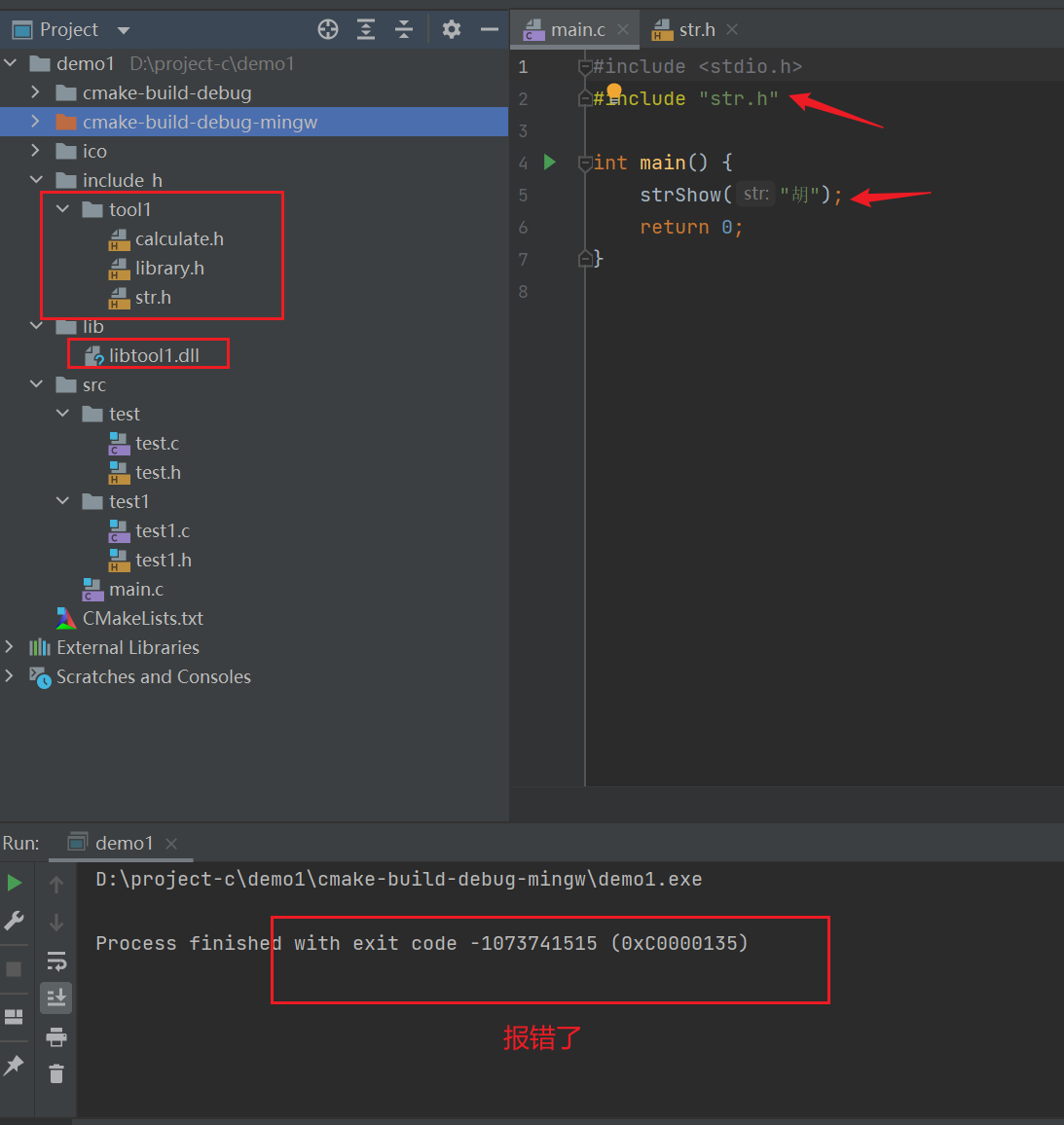
C语言-模块化-Clion(静态库,动态库)使用
保姆级教程:Azkaban执行jar包(带测试样例及结果)
Can you write the software test questions?
Graphic network: uncover the principle behind TCP's four waves, combined with the example of boyfriend and girlfriend breaking up, which is easy to understand

《通信软件开发与应用》课程结业报告

随机推荐
Direct addition is more appropriate
SQLite3 data storage location created by Android
牛熊周期与加密的未来如何演变?看看红杉资本怎么说
如何用Diffusion models做interpolation插值任务?——原理解析和代码实战
Kwai applet guaranteed payment PHP source code packaging
mysql/mariadb怎样生成core文件
Introduction to ADB tools
Apache多个组件漏洞公开(CVE-2022-32533/CVE-2022-33980/CVE-2021-37839)
PHP 计算个人所得税
系统测试的类型有哪些,我给你介绍
#797div3 A---C
Clickhouse principle analysis and application practice "reading notes (8)
Give some suggestions to friends who are just getting started or preparing to change careers as network engineers
Remote Sensing投稿经验分享
Vim 字符串替换
力扣5_876. 链表的中间结点
Ml backward propagation
Remote Sensing投稿經驗分享
Talk about the realization of authority control and transaction record function of SAP system
[error] error loading H5 weight attributeerror: 'STR' object has no attribute 'decode‘