当前位置:网站首页>Ml self realization / linear regression / multivariable
Ml self realization / linear regression / multivariable
2022-07-08 01:58:00 【xcrj】
principle
Prediction function :
h θ ( x ) = θ 0 + θ 1 x 1 + θ 2 x 2 + θ 3 x 3 h_\theta(x)=\theta_0+\theta_1x_1+\theta_2x_2+\theta_3x_3 hθ(x)=θ0+θ1x1+θ2x2+θ3x3
Parameters :
θ 0 , θ 1 , θ 2 , θ 3 \theta_0, \theta_1, \theta_2, \theta_3 θ0,θ1,θ2,θ3
cost function : Least square method
J ( θ 0 , θ 1 , θ 2 , θ 3 ) = 1 m ∑ i = 1 m ( h θ ( x ( i ) ) − y ( i ) ) 2 J(\theta_0,\theta_1,\theta_2,\theta_3)=\frac{1}{m}\sum\limits_{i=1}^m(h_\theta(x^{(i)})-y^{(i)})^2 J(θ0,θ1,θ2,θ3)=m1i=1∑m(hθ(x(i))−y(i))2
The goal is :
m i n i m i z e θ 0 , θ 1 , θ 2 , θ 3 J ( θ 0 , θ 1 , θ 2 , θ 3 ) \mathop{minimize}\limits_{\theta_0,\theta_1,\theta_2,\theta_3}J(\theta_0,\theta_1,\theta_2,\theta_3) θ0,θ1,θ2,θ3minimizeJ(θ0,θ1,θ2,θ3)
Batch gradient descent algorithm :
- Repeat until it converges {
θ j : = θ j − α ∂ J ( θ 0 , θ 1 , θ 2 , θ 3 ) ∂ θ j \theta_j:=\theta_j-\alpha\frac{\partial{J(\theta_0,\theta_1,\theta_2,\theta_3)}}{\partial{\theta_j}} θj:=θj−α∂θj∂J(θ0,θ1,θ2,θ3)
} - Repeat until it converges {
θ 0 : = θ 0 − α 2 m ∑ i = 1 m ( h θ ( x ( i ) ) − y ( i ) ) \theta_0:=\theta_0-\alpha\frac{2}{m}\sum\limits_{i=1}^m(h_\theta(x^{(i)})-y^{(i)}) θ0:=θ0−αm2i=1∑m(hθ(x(i))−y(i))
θ 1 : = θ 1 − α 2 m ∑ i = 1 m ( h θ ( x ( i ) ) − y ( i ) ) ⋅ x ( i ) \theta_1:=\theta_1-\alpha\frac{2}{m}\sum\limits_{i=1}^m(h_\theta(x^{(i)})-y^{(i)})\cdot{x^{(i)}} θ1:=θ1−αm2i=1∑m(hθ(x(i))−y(i))⋅x(i)
θ 2 : = θ 2 − α 2 m ∑ i = 1 m ( h θ ( x ( i ) ) − y ( i ) ) ⋅ x ( i ) \theta_2:=\theta_2-\alpha\frac{2}{m}\sum\limits_{i=1}^m(h_\theta(x^{(i)})-y^{(i)})\cdot{x^{(i)}} θ2:=θ2−αm2i=1∑m(hθ(x(i))−y(i))⋅x(i)
θ 3 : = θ 3 − α 2 m ∑ i = 1 m ( h θ ( x ( i ) ) − y ( i ) ) ⋅ x ( i ) \theta_3:=\theta_3-\alpha\frac{2}{m}\sum\limits_{i=1}^m(h_\theta(x^{(i)})-y^{(i)})\cdot{x^{(i)}} θ3:=θ3−αm2i=1∑m(hθ(x(i))−y(i))⋅x(i)
} - Be careful : Batch gradient descent algorithm needs to be updated at the same time θ 0 , θ 1 , θ 2 , θ 3 \theta_0,\theta_1,\theta_2,\theta_3 θ0,θ1,θ2,θ3
Normal equation method :
- X θ = y ⇒ X − 1 y = θ ⇒ ( X T X ) − 1 X T y = θ X\theta=y\Rightarrow X^{-1}y=\theta\Rightarrow(X^TX)^{-1}X^Ty=\theta Xθ=y⇒X−1y=θ⇒(XTX)−1XTy=θ
Experience
Gradient descent learning rate α \alpha α choice
- α \alpha α Too small , Convergence to the optimal speed is slow
- α \alpha α Too big , May miss the best , It won't converge
- α = . . . , 0.001 , 0.003 , 0.01 , 0.03 , 0.1 , 0.3 , 1 , . . . \alpha=..., 0.001, 0.003, 0.01, 0.03, 0.1, 0.3, 1, ... α=...,0.001,0.003,0.01,0.03,0.1,0.3,1,...
- Try α \alpha α, find max α \alpha α,min α \alpha α, They all make cost Step down , stay min and max α \alpha α Fine tuning in
Normal equation method - X − 1 X^{-1} X−1 There is no problem
- Remove similar features
- The number of features > Characteristic dimension , Features must be linearly correlated , Some features can be deleted
Gradient descent and normal equation method selection
| contrast | Gradient descent algorithm | Normal equation algorithm |
|---|---|---|
| Learning rate | need | Unwanted |
| The number of iterations | n Time | 1 Time |
| Characteristic quantity | >0 | <1000000, Because the time complexity of matrix calculation is O ( n 3 ) O(n^3) O(n3) |
| adaptive | Various models | linear regression model |
Data sets
- features : Number of cylinders (cylinders), displacement (displacement), horsepower (horsepower), weight (weights), The acceleration (acceleration) wait
- The goal is :mpg(mile per gallon)-1 Miles per gallon
- This paper is multivariable linear regression , The discussion is characterized by acceleration, displacement, horsepower; The goal is MPG The situation of
Code
import pandas as pd
import seaborn as sns
import numpy as np
import matplotlib
import matplotlib.pyplot as plt

matplotlib.rcParams['font.family'] = 'STSong'
matplotlib.rcParams['font.size'] = 20


class DataSet(object):
    """ X_train  Training set samples  y_train  Training set sample value  X_test  Test set samples  y_test  Test set sample values  """

    def __init__(self, X_train, y_train, X_test, y_test):
        self.X_train = X_train
        self.y_train = y_train
        self.X_test = X_test
        self.y_test = y_test


def read_data():
    """  Reading data  """
    column_names = ['MPG', 'cylinders', 'displacement', 'horsepower', 'weight', 'acceleration', 'model year', 'origin']
    # names: Header
    # sep: Separator
    # skipinitialspace: Ignore the space after the delimiter
    # comment: Ignore \t Note after
    # na_values: Use ? Replace NA Value
    origin_data = pd.read_csv("./data/auto-mpg.data", names=column_names, sep=" ", skipinitialspace=True, comment="\t",
                              na_values="?")
    #  Copy
    data = origin_data.copy()
    # tail() Print last n Row data
    print(data.tail())
    return data


def clean_data(data):
    """  Data cleaning : Handling outliers  """
    # dataset Does it contain NA data
    # pandas 0.22.0+ Only then isna(), Upgrade order :pip install --upgrade pandas==0.22.0
    print('NA Row number :', data.isna().sum())
    #  Delete the exception line
    cleaned_data = data.dropna()
    return cleaned_data


def split_data(data):
    """  Divide the data   Divided into train, test;train Used to train the prediction function ,test Used to test the predicted function value and y_test Distance of   This code does multivariable linear regression : X= Number of cylinders (cylinders), displacement (displacement), horsepower (horsepower), weight (weights), The acceleration (acceleration) 'cylinders', 'displacement', 'horsepower', 'weight', 'acceleration', 'model year', 'origin' y=MPG(mile per gallon-1 Gallons can run miles ) """
    copied_data = data.copy()
    # frac: The proportion of rows extracted ;random_state  Random seeds
    train_dataset = copied_data.sample(frac=0.8, random_state=1)
    #  Take the rest of the test set
    test_dataset = copied_data.drop(train_dataset.index)

    column_list = ['cylinders', 'displacement', 'horsepower']
    X_train = train_dataset[column_list]
    y_train = train_dataset[['MPG']]
    X_test = test_dataset[column_list]
    y_test = test_dataset[['MPG']]
    dataset = DataSet(X_train, y_train, X_test, y_test)

    return dataset


def check_dataset(dataset):
    """  Check the dataset   Check the distribution   Check the overall situation  """
    #  The relationship between the two characteristics
    sns.pairplot(dataset.X_train, diag_kind="kde")
    sns.pairplot(dataset.y_train, diag_kind="kde")
    sns.pairplot(dataset.X_test, diag_kind="kde")
    sns.pairplot(dataset.y_test, diag_kind="kde")
    plt.show()

    print(dataset.X_train.describe().transpose())
    print(dataset.y_train.describe().transpose())
    print(dataset.X_test.describe().transpose())
    print(dataset.y_test.describe().transpose())


def mean_normalize(dataset):
    """  Normalization of eigenvalue mean   Make the contour map composed of different features more round , The gradient descent speed from any direction is almost the same   Eigenvalues affect the rate of gradient descent ( Slender contour map ) """
    #  mean value
    # axis=0, Find the average value of each column , Output as a line
    mu = np.mean(dataset.X_train, axis=0)
    #  Standard deviation
    sigma = np.std(dataset.X_train, axis=0)
    X_train_norm = (dataset.X_train - mu) / sigma

    mu = np.mean(dataset.X_test, axis=0)
    #  Standard deviation
    sigma = np.std(dataset.X_test, axis=0)
    X_test_norm = (dataset.X_test - mu) / sigma
    dataset_norm = DataSet(X_train_norm, dataset.y_train, X_test_norm, dataset.y_test)
    return dataset_norm


class LinearRegression(object):
    """  Multivariate linear regression   Gradient descent algorithm  """

    def __init__(self):
        """  This experiment takes 3 Features  """
        # theta0 yes bias
        self.theta0 = 0
        # theta
        self.theta = np.array([[0, 0, 0]]).T

    def gradient_descent(self, X, y, alpha=0.001, num_iter=100):
        """  Gradient descent algorithm , Least square method  :param X: X_train,  Multivariate linear regression  x_1,x_2,x_3 :param y: y_train :param alpha:  Learning rate , Adjust the step size of a gradient descent  :param num_iter:  The number of iterations  """
        # m Is the number of samples
        m, _ = X.shape
        costs = []
        for i in range(num_iter):
            #  Predictive value
            h = self.theta0 + np.dot(X, self.theta)
            #  Costing
            cost = (1 / m) * np.sum((h - y) ** 2)
            costs.append(cost)

            #  Gradient calculation
            dJ_dtheta0 = (2 / m) * np.sum(h - y)
            dJ_dtheta = (2 / m) * np.dot((h - y).T, X).T

            #  Simultaneous updating theta1 and theta0
            self.theta0 = self.theta0 - alpha * dJ_dtheta0
            self.theta = self.theta - alpha * dJ_dtheta

        return costs

    def normal_equation(self, X, y):
        """  Normal equation method  """
        self.theta_ne = np.dot(np.dot(np.linalg.inv(np.dot(X.T, X)), X.T), y)
        self.theta_ne0 = 0

    def show_train(self, costs, num_iter):
        """  Show the training process  """
        fig = plt.figure(figsize=(10, 6))
        plt.plot(np.arange(num_iter), costs)
        plt.title(" Cost changes ")
        plt.xlabel(" The number of iterations ")
        plt.ylabel(" cost ")
        plt.show()

    def hypothesis(self, X, theta0, theta):
        """  Prediction function  """
        return theta0 + np.dot(X, theta)


def evaluate_model(y_test, h):
    """  Evaluation model  """
    # MSE: Mean square error
    print("MSE: %f" % (np.sum((h - y_test) ** 2) / len(y_test)))
    # RMSE: Root mean square difference
    print("RMSE: %f" % (np.sqrt(np.sum((h - y_test) ** 2) / len(y_test))))


def main():
    #  Reading data
    data = read_data()
    #  Data cleaning
    cleaned_data = clean_data(data)
    #  Split data
    dataset = split_data(cleaned_data)
    #  Check the dataset
    # check_dataset(dataset)
    #  Mean normalization , Eigenvalues affect the rate of gradient descent ( Slender contour map )
    dataset_norm = mean_normalize(dataset)
    print('#### Gradient descent algorithm ####')
    #  Build the model
    linear_regression = LinearRegression()
    num_iteration = 100
    # dataframe.values Method pandas/DataFrame turn numpy/ndarray
    costs = linear_regression.gradient_descent(dataset_norm.X_train.values, dataset_norm.y_train.values, alpha=0.03,
                                               num_iter=num_iteration)
    #  Show the training process
    linear_regression.show_train(costs, num_iteration)
    #  Evaluation model , Evaluate the prediction function
    h = linear_regression.hypothesis(dataset_norm.X_test.values, linear_regression.theta0, linear_regression.theta)
    evaluate_model(dataset_norm.y_test.values, h)
    print('#### Normal equation algorithm ####')
    linear_regression.normal_equation(dataset_norm.X_train.values, dataset_norm.y_train.values)
    h = linear_regression.hypothesis(dataset_norm.X_test.values, linear_regression.theta_ne0,
                                     linear_regression.theta_ne)
    evaluate_model(dataset_norm.y_test.values, h)


if __name__ == '__main__':
    main()
边栏推荐
- Nanny level tutorial: Azkaban executes jar package (with test samples and results)
- Chapter 7 behavior level modeling
- 软件测试笔试题你会吗?
- Keras深度学习实战——基于Inception v3实现性别分类
- 保姆级教程:Azkaban执行jar包(带测试样例及结果)
- Mouse event - event object
- burpsuite
- 《ClickHouse原理解析与应用实践》读书笔记(7)
- ClickHouse原理解析与应用实践》读书笔记(8)
- Codeforces Round #643 (Div. 2)——B. Young Explorers
猜你喜欢

如何制作企业招聘二维码?
ANSI / nema- mw- 1000-2020 magnetic iron wire standard Latest original

Chapter 7 behavior level modeling
#797div3 A---C
静态路由配置全面详解,静态路由快速入门指南

生态 | 湖仓一体的优选:GBase 8a MPP + XEOS
Nacos microservice gateway component +swagger2 interface generation
【目标跟踪】|DiMP: Learning Discriminative Model Prediction for Tracking
Get familiar with XML parsing quickly
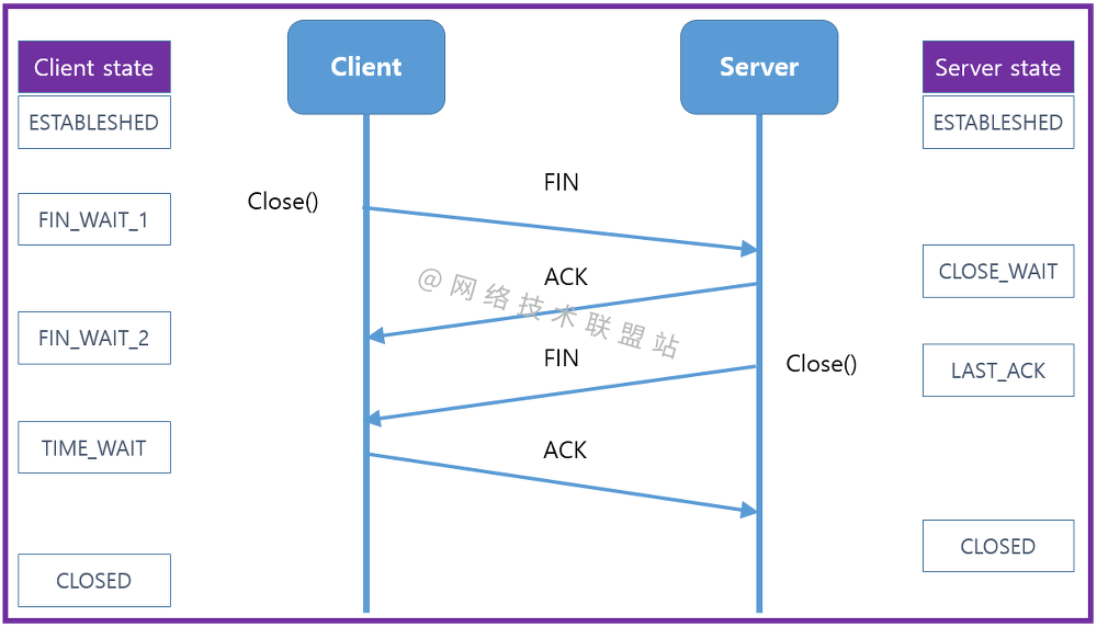
图解网络:揭开TCP四次挥手背后的原理,结合男女朋友分手的例子,通俗易懂
随机推荐
Node JS maintains a long connection
PHP calculates personal income tax
分布式定时任务之XXL-JOB
WPF 自定义 写实风 雷达图控件
adb工具介绍
Remote Sensing投稿经验分享
Clickhouse principle analysis and application practice "reading notes (8)
保姆级教程:Azkaban执行jar包(带测试样例及结果)
系统测试的类型有哪些,我给你介绍
How to realize batch control? MES system gives you the answer
电路如图,R1=2kΩ,R2=2kΩ,R3=4kΩ,Rf=4kΩ。求输出与输入关系表达式。
从Starfish OS持续对SFO的通缩消耗,长远看SFO的价值
Js中forEach map无法跳出循环问题以及forEach会不会修改原数组
Urban land use distribution data / urban functional zoning distribution data / urban POI points of interest / vegetation type distribution
Redisson distributed lock unlocking exception
Nmap tool introduction and common commands
Mouse event - event object
微信小程序uniapp页面无法跳转:“navigateTo:fail can not navigateTo a tabbar page“
ArrayList源码深度剖析,从最基本的扩容原理,到魔幻的迭代器和fast-fail机制,你想要的这都有!!!
Version 2.0 of tapdata, the open source live data platform, has been released