Brief analysis of tensorboard visual processing cases

https://tensorflow.google.cn/tensorboard?hl=zh-cn

TensorBoard Provide visualization functions and tools needed for machine learning experiments ：
Track and visualize indicators such as loss and accuracy
Visual model diagram （ Operations and layers ）
See the weight 、 Histograms of deviations or other tensors over time
Project the embedding into the lower dimensional space
display picture 、 Text and audio data
analyse TensorFlow Program
And more

TensorBoard It's a separate package （ No pytorch Medium ）, The purpose of this package is to visualize the various parameters and results in your model .

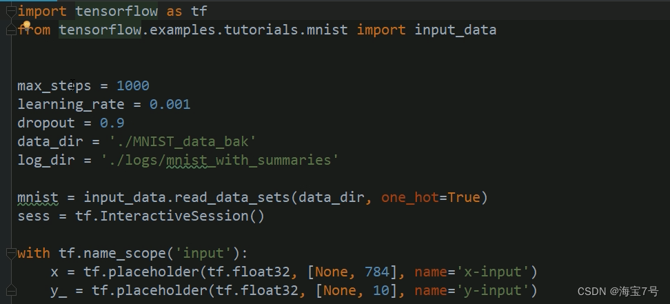
Code attached ：

import tensorflow as tf
from tensorflow.examples.tutorials.mnist import input_data


max_steps = 1000
learning_rate = 0.001
dropout = 0.9
data_dir = './MNIST_data_bak'
log_dir = './logs/mnist_with_summaries'

mnist = input_data.read_data_sets(data_dir, one_hot=True)
sess = tf.InteractiveSession()

with tf.name_scope('input'):
    x = tf.placeholder(tf.float32, [None, 784], name='x-input')
    y_ = tf.placeholder(tf.float32, [None, 10], name='y-input')

with tf.name_scope('input_reshape'):
    # 784 The dimension is deformed to keep the image to the node 
    # -1  Represents the number of pictures coming in 、28,28 Is the height and width of the picture ,1 Is the color channel of the picture 
    image_shaped_input = tf.reshape(x, [-1, 28, 28, 1])
    tf.summary.image('input', image_shaped_input, 10)


#  Define the initialization method of neural network 
def weight_variable(shape):
    initial = tf.truncated_normal(shape, stddev=0.1)
    return tf.Variable(initial)


def bias_variable(shape):
    initial = tf.constant(0.1, shape=shape)
    return tf.Variable(initial)


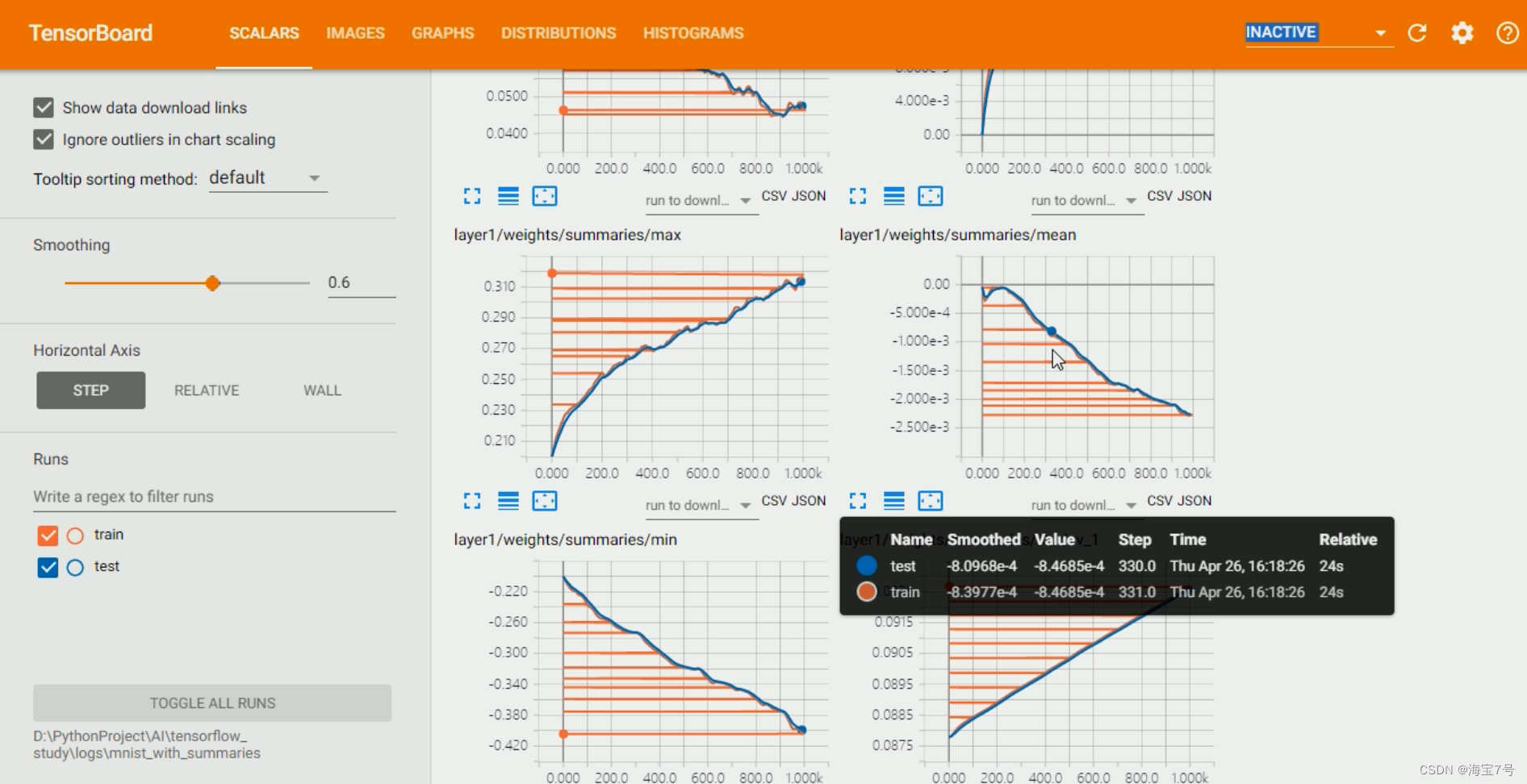
#  Definition Variable Variable data summary function , We calculate the mean、stddev、max、min
#  Use... For these scalar data tf.summary.scalar Record and summarize 
#  Use tf.summary.histogram Record variables directly var Histogram data 
def variable_summaries(var):
    with tf.name_scope('summaries'):
        mean = tf.reduce_mean(var)
        tf.summary.scalar('mean', mean)
        with tf.name_scope('stddev'):
            stddev = tf.sqrt(tf.reduce_mean(tf.square(var - mean)))
        tf.summary.scalar('stddev', stddev)
        tf.summary.scalar('max', tf.reduce_max(var))
        tf.summary.scalar('min', tf.reduce_min(var))
        tf.summary.histogram('histogram', var)


#  To design a MLP Multilayer neural network to train data 
#  The model data is summarized in each layer 
def nn_layer(input_tensor, input_dim, output_dim, layer_name, act=tf.nn.relu):
    with tf.name_scope(layer_name):
        with tf.name_scope('weights'):
            weights = weight_variable([input_dim, output_dim])
            variable_summaries(weights)
        with tf.name_scope('biases'):
            biases = bias_variable([output_dim])
            variable_summaries(biases)
        with tf.name_scope('Wx_plus_b'):
            preactivate = tf.matmul(input_tensor, weights) + biases
            tf.summary.histogram('pre_activations', preactivate)
        activations = act(preactivate, name='activation')
        tf.summary.histogram('activations', activations)
        return activations


#  We use the function just defined to create a neural network , The input dimension is the size of the picture 784=28*28
#  The output dimension is the number of hidden nodes 500, Create another Dropout layer , And use tf.summary.scalar Record keep_prob
#  And then use nn_layer Define the neural network output layer , Its input dimension is the number of hidden nodes in the upper layer 500, The output dimension is the number of categories 10
#  At the same time, the activation function is congruent mapping identity, Temporarily not used softmax
hidden1 = nn_layer(x, 784, 500, 'layer1')

with tf.name_scope('dropout'):
    keep_prob = tf.placeholder(tf.float32)
    tf.summary.scalar('dropout_keep_probability', keep_prob)
    dropped = tf.nn.dropout(hidden1, keep_prob)

y = nn_layer(dropped, 500, 10, 'layer2', act=tf.identity)

#  Use tf.nn.softmax_cross_entropy_with_logits() Analyze the results of the previous output layer Softmax
#  Process and calculate the cross entropy loss cross_entropy, Calculate the average loss , Use tf.summary.scalar Make statistical summary 
with tf.name_scope('cross_entropy'):
    diff = tf.nn.softmax_cross_entropy_with_logits(logits=y, labels=y_)
    with tf.name_scope('total'):
        cross_entropy = tf.reduce_mean(diff)
tf.summary.scalar('cross_entropy', cross_entropy)


#  Use Adam The optimizer optimizes the loss , At the same time, the number of correctly predicted samples is counted and the accuracy rate is calculated accuracy, Summary 
with tf.name_scope('train'):
    train_step = tf.train.AdamOptimizer(learning_rate).minimize(cross_entropy)
with tf.name_scope('accuracy'):
    with tf.name_scope('correct_prediction'):
        correct_prediction = tf.equal(tf.argmax(y, 1), tf.argmax(y_, 1))
    with tf.name_scope('accuracy'):
        accuracy = tf.reduce_mean(tf.cast(correct_prediction, tf.float32))

tf.summary.scalar('accuracy', accuracy)

#  Because we have defined too many tf.summary Summary operation , It is too troublesome to perform these operations one by one ,
#  Use tf.summary.merge_all() Get all summary operations directly , For later execution 
merged = tf.summary.merge_all()
#  Define two tf.summary.FileWriter The file recorder has different subdirectories , It is used to store the log data of training and testing respectively 
train_writer = tf.summary.FileWriter(log_dir + '/train', sess.graph)
test_writer = tf.summary.FileWriter(log_dir + '/test')
#  meanwhile , take Session Calculation chart sess.graph Join the training process , So again TensorBoard Of GRAPHS It can be displayed in the window 
#  Visualization of the whole calculation diagram , Finally, initialize all variables 
tf.global_variables_initializer().run()


#  Definition feed_dict function , If it's training , Need to set up dropout, If it's a test ,keep_prob Set to 1
def feed_dict(train):
    if train:
        xs, ys = mnist.train.next_batch(100)
        k = dropout
    else:
        xs, ys = mnist.test.images, mnist.test.labels
        k = 1.0
    return {
    x: xs, y_: ys, keep_prob: k}


#  Executive Training 、 test 、 Logging operations 
#  Save the model created by 
saver = tf.train.Saver()
for i in range(max_steps):
    if i % 10 == 0:
        summary, acc = sess.run([merged, accuracy], feed_dict=feed_dict(False))
        test_writer.add_summary(summary, i)
        print('Accuracy at step %s: %s' % (i, acc))
    else:
        if i % 100 == 99:
            run_options = tf.RunOptions(trace_level=tf.RunOptions.FULL_TRACE)
            run_metadata = tf.RunMetadata()
            summary, _ = sess.run([merged, train_step], feed_dict=feed_dict(True))
            train_writer.add_run_metadata(run_metadata, 'step%03d' % i)
            train_writer.add_summary(summary, 1)
            saver.save(sess, log_dir + 'model.ckpt', i)
            print('Adding run metadata for', i)
        else:
            summary, _ = sess.run([merged, train_step], feed_dict=feed_dict(True))
            train_writer.add_summary(summary, i)

train_writer.close()
test_writer.close()

Training process

Advanced usage operations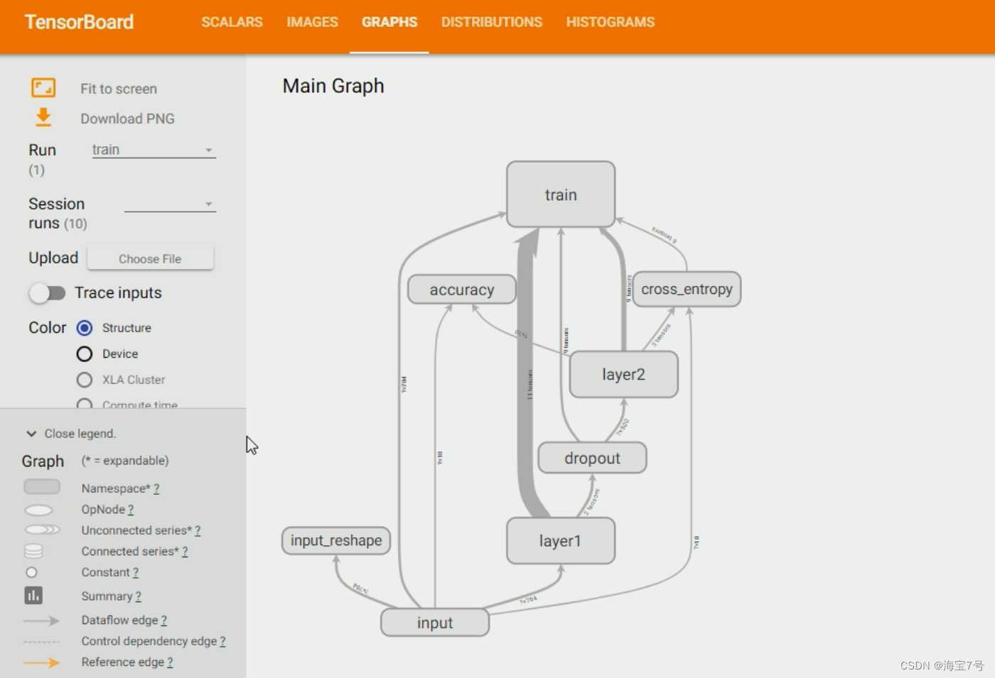


Personally feel , Still need self-study , Or there is a leader , Otherwise, the starting process and subsequent processing are more troublesome .
TensorBoard Visual tools simple tutorial reference
https://blog.csdn.net/qq_41573860/article/details/106674370

long-range tensorboard

Because of the conditions , Usually, deep learning is conducted on a remote server , utilize SSH Direction Tunnel Technology , Forward the port data on the server to the corresponding local port , Then you can log data on the local method server .
Reference resources ：https://blog.csdn.net/zhaokx3/article/details/70994350