当前位置:网站首页>Learn face detection from scratch: retinaface (including magic modified ghostnet+mbv2)
Learn face detection from scratch: retinaface (including magic modified ghostnet+mbv2)
2022-07-08 02:18:00 【pogg_】
Learn face detection from scratch Retinaface piece ( Contains magic revision )
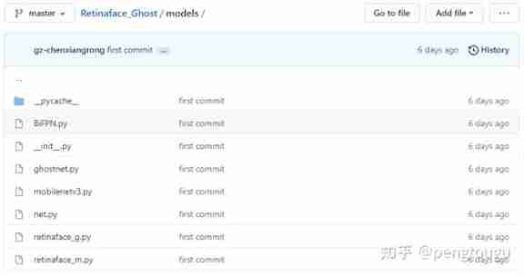
The code is open source , Welcome white whoring and star:
github.com/pengtougu/Retinaface_Ghost
One 、 Interpretation of the thesis
The study of the thesis is conducted by Sansa Boss finished :
https://www.zhihu.com/people/0e4e23de534ba625a13b39a3153fa942
Preface
Retinaface yes Insightface Team in 2019 The new face detection model proposed in , The model is in WiderFace The data set is refreshed AP. The source code is open source insightface, The original model uses mxnet Build the framework , At present, the community also has other versions of the framework , Nothing is better known than pytorch Version of retinaface.Retinaface It is based on detection network RetinaNet Improved version ( you 're right , and centerface be based on centernet similar ), Added SSH The three-level detection module of the network , Improve the detection accuracy . The author provides two versions of the network (mobilenet and resnet), be based on MobileNet The build of is designed to provide faster detection , be based on ResNet The build version of is more important than the index of accuracy .
Abstract :
Although great progress has been made in face detection with single scene , But it is still a challenge to locate the face accurately and effectively in natural scenes . This paper presents a powerful single order face detector , We call it RetinaFace, The detector passes the joint external supervision (extra-supervised) And self supervision (self-supervised) Multi task learning , Carry out pixel level positioning for faces of various sizes .
say concretely , We have made contributions in the following five aspects .
(1) stay WIDER FACE Five facial keys are manually marked on the dataset , With the help of external supervision signal, the difficult face detection is significantly improved .
(2) Added a self supervised grid coding Branch , Used to predict a pixel by pixel 3D Face information , And make the branch parallel to the existing supervised Branch .
(3) stay WIDER FACE Hard test set .RetinaFace Better than the most advanced average accuracy (AP) Higher than 1.1%( achieve AP be equal to 91.4%, finger ISRN)
(4) stay IJB-C Test set ,RetinaFace Make the best face feature extraction model at that time ArcFace In face authentication (face verification) The performance of is further improved (TAR=89.59 FAR=1e-6)
(5) Adopt lightweight backbone network ,RetinaFace Can be in a single CPU Run in real time .
Introduce
Different from the general target detection method , The feature aspect ratio of face detection changes little (1:1 To 1:1.5), But the scale changes greatly ( A picture contains multiple faces , From a few pixels to thousands of pixels ). Recently, the best method focuses on single-stage design , Conduct dense face position and scale sampling on the feature pyramid , Compared with the two-stage cascade method , This design has achieved good performance and speed improvement . Follow this route , Our improved single-level face detection framework , And by using the multi task loss of strong supervision and self supervision models , The best dense face location method at present is proposed . The thought is shown in the picture :

The single-level pixel by pixel face location method utilizes external supervised and self supervised multi task learning, including face frame classification and regression branches at the same time . Every positive anchor Output : Face score , Face frame ,5 Personal face key points , Projected onto a plane 3D Face vertex
stay Mask R-CNN【1】 in , By adding the branches submerged by the target and parallel with the detection box recognition and regression branches , The detection performance is significantly improved . This proves that dense pixel level annotation is also useful for improving detection performance . However ,WIDER FACE The part of face that is difficult to detect in cannot obtain face annotation information . Since the supervision signal is not easy to obtain , Then the question becomes whether we can use unsupervised methods to further improve face detection .
FAN【2】 Propose a anchor Level attention map to improve occluded face detection , However , The proposed attention map is rough and does not contain semantic information . lately , Self supervision 3D The deformation model has achieved good results in natural scenes 3D Face . Special ,Mesh Decoder【3】 The super real-time speed is obtained by image convolution on shape and texture , However , take mesh decoder The biggest challenge when applied to single-stage detectors is :(1) Camera parameters are difficult to estimate accurately (2) Joint potential shape and texture estimation is predicted from a simple feature vector ( On the characteristic pyramid 1x1 Convolution ) Not through RoI Pooling characteristics , In this way, there is a risk of feature drift . This paper uses network coding (mesh decoder), Predict a pixel level through self supervised learning 3D Face shape , Parallel with existing supervision branches .
All in all , The paper puts forward several main contributions :
- Based on single-stage design , A new pixel level face location method is proposed RetinaFace, Use multi task learning strategy to predict face score at the same time , Face frame ,5 Key points and corresponding to each face pixel 3D Location .
- stay WIDER FACE Data hard On a subset ,RetinaFace Of AP=91.4%, Better than the best two-stage cascade method ISRN【4】 promote 1.1%
- stay IJB-C Test set ,RetinaFace take ArcFace In face authentication (face verification) Further improve (TAR=89.59%,FAR=1e-6), This means that better face location can significantly improve face recognition
- By using lightweight skeleton network ,RetinaFace Can be in a single CPU The last one VGA Resolution images run in real time
| VGA | HD | 4K |
|---|---|---|
| 640×480 | 1920×1080 | 4096×2160 |
- Annotation and source code
https://zhuanlan.zhihu.com/p/101600780
Related work
Image pyramid vs Characteristic pyramid : The sliding window strategy dates back decades . Milestone work is Viola-Jones Cascade is proposed to reject face false detection in image pyramid and pursue real-time , Leading the wide reference of scale invariant face detection framework . Although the sliding window on the image pyramid is the main detection method , With the appearance of characteristic pyramids , Sliding on multiple scale feature maps anchor It is quickly applied to face detection .
Double order vs Single order : The current face detection methods inherit the results of some common detection methods , There are two main categories : Two order methods such as Faster RCNN And single order methods such as SSD and RetinaNet. The second-order method applies a “proposal and refinement” Mechanism extraction and high precision positioning . However, the single order method samples the position and scale of human face intensively , The positive and negative samples that lead to extreme imbalance in the training process . To deal with this imbalance ,unsample and facal loss Widely used . Compared with the two order method , Single order method is more efficient and has higher recall rate , But there is a risk of higher false positives , Affect the positioning accuracy .
Context modeling : In order to enhance the context reasoning ability of the model to small face ,SSH and PyramidBox In the feature pyramid, the context module is used to enhance the receptive field in Euclidean grid . To enhance CNN The ability to simulate non strict transformations of , Deformed convolution networks (DCN) Using a new deformation layer to simulate geometric deformation .WIDER Face Challenge 2018 For face detection , Strictly ( expand ) And not strictly ( deformation ) Context modeling is complementary and orthogonal .
Multi task learning : The combination of face detection and alignment is widely used , This is because the aligned face can provide better features for face classification . stay Mask R-CNN in , By adding a parallel branch of the prediction target mask , Detection performance has been significantly improved .Densepose utilize Mask-RCNN The architecture of , To get dense labels and locations for each selection area . For all that , Dense regression tags are trained by supervised learning . Besides ,dense The branch is a very small FCN The Internet , Apply to every one of them RoI To predict pixel to pixel dense mapping .
RetinaFace principle
See sansa Big guy's blog , I won't go into details here
https://zhuanlan.zhihu.com/p/103005911
Experimental part
4.1 Data sets
WIDER FACE Data set containing 32,203 Two images and 393,703 Personal face frame , scale , Posture , expression , Both occlusion and illumination change greatly .WIDER FACE Data sets are divided into training 40% verification 10% And testing 50% Three subsets , By means of 61 Random sampling in scene classification . be based on EdgeBox The detection rate of , By incrementally merging difficult samples , The degree of difficulty is divided into 3 level : Easy to , Neutral and difficult .
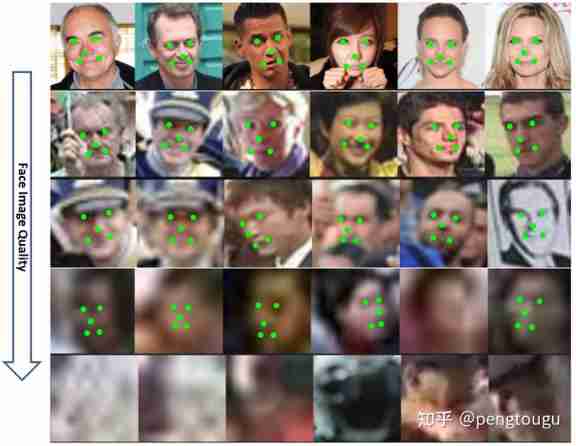
Extra annotation : Pictured 4 And table 1, We define 5 Personal face quality level , Mark the difficulty according to the key points of the face and mark 5 A key point ( Eye Center , Nose , corners of the mouth ). We marked a total of 84.6k A training set of faces and 18.5k Verification set faces .

4.2 Application details

Characteristic pyramid RetinaFace Apply feature pyramids from P2 To P6, among P2 To P5 It's from Resnet Residual level (C2 To C5) Come by calculation .P6 take C5 Through one 3x3,s=2 The convolution of is obtained .C1 To C5 From in ImageNet-11k Pre trained on dataset ResNet-152 Classification framework and P6 adopt Xavier Random initialization .
Context module Inspired by SSH and PyramidBox, We also apply the independent context module to 5 Feature pyramids are used to improve receptive fields and enhance strict context modeling . from WIDER Face Challenge 2018 Summarize experience , We will connect all the side 3x3 The convolution layer and the context module are replaced by DCN【6】, It can further strengthen the ability of non strict context modeling
Loss of head (Loss Head) For all negative samples anchors, Only classification loss is used . For positive samples anchors, Then calculate the multi task loss . We are between different characteristic graphs H n ∗ W n ∗ 256 , n ∈ 2 , . . . , 6 H_{n}*W_{n}*256,n∈{2, . . . , 6} Hn∗Wn∗256,n∈2,...,6 Use a shared loss header (1x1 Convolution ). For grid coding , We use a pre training model 【3】, The computational overhead is small .
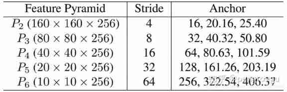
Anchor Set up As shown in the table 2 Shown , In from P2 To P6 Use specific scales on the pyramid of features anchor.P2 For grabbing small faces , By using smaller anchor, Of course , The calculation cost will increase and the false detection will increase . Set the scale step size to 2 1 / 3 2^{1/3} 21/3( I don't understand here , Mark it first ), Aspect ratio 1:1. The input image 640x640,anchor from 16x16 To 406x406 On the characteristic pyramid . All in all 102,300 individual anchors,75% come from P2 layer . Explain this to you 102300 How did it come from :(160160+8080+4040+2020+10)*3(SSH There are three floors )= 102300.
In the training phase ground-truth Of IOU Greater than 0.5 Of anchor The target is a positive sample , Less than 0.3 Of anchor Think it's the background .anchors There is >99% All of them are negative samples , Use standards OHEM Avoid the imbalance between positive and negative samples . adopt loss Value selection negative sample , Positive sample ratio 1:3
Data to enhance WIDER FACE Yes 20% My little face , Random from the original image crop square patch And zoom to 640*640 To generate a larger face . square patch The interception rule of is , Random selection [0.3,1] Scale the length of the short side of the original image . stay crop Faces on the border , The retention center is crop patch Inside the face frame . Except random crop, We rotate half of the image horizontally and disturb the symmetrical color .
Training details Use SGD Optimizer training RetinaFace(momentum=0.9,weight decay = 0.0005,batchsize=8x4),Nvidia Tesla P40(24G) GPUs. Initial learning rate 0.001,5 individual epoch After a 0.01, Then in the first 55 And the 68 individual epoch Time divided by 10.
Test details stay WIDER FACE Up test , Take advantage of flip And multiscale ( Select the short edge of the image , The size is in 【500,800,1100,1400,1700】 Between ) Strategy . Use IoU threshold 0.4, The voting strategy is used to predict the set of face frames .
4.3 Ablation Experiment
Superimposed tricks Several models of WIDER FACE On the verification set AP and mAP Such as the table 3 Shown . By using FPN、 Context information 、 Deformation convolution and other strategies , Got a good baseline. By increasing the 5 Point Branch , stay hard Significantly improved on subset samples , explain 5 The improvement of point-to-point face detection is obvious . In contrast , Dense regression branches have increased easy and medium Subset face detection , But yes. hard The improvement of subset faces is not great . hold 5 Point branches are used with dense branches , Performance is still improved .
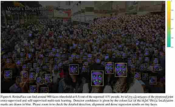
4.4 Face frame accuracy
Pictured 6 Shown , It shows the detection quality in the case of dense faces , stay 0.5 The above faces are detected 900 individual , The total is 1151 Face . In addition to the accuracy of the face frame ,5 Point positioning is also robust under different pose occlusion resolutions . Although there are still cases of failure in dense face location under severe occlusion , But it works well on some clear adult faces .
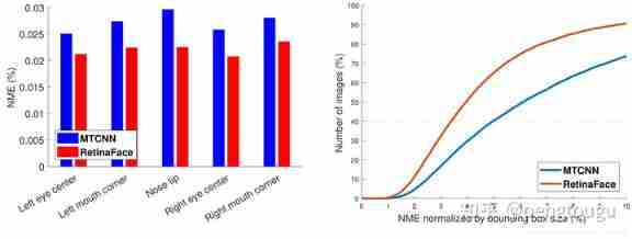
4.5 Five point positioning accuracy
To evaluate the accuracy of five point positioning , We are AFLW On dataset (24386 Face ) and WIDER FACE Verification set (18.5k Face ) Comparison of the MTCNN and RetinaFace. Normalize the distance using the face frame size . Pictured 7a Shown , Given in AFLW The average error of each point on .RetinaFace Normalize the average error NME from MTCNN Of 2.72% Down to 2.21%. In the figure 7b in , Show the WIDER FACE The cumulative error distribution on the verification set CED. And MTCNN comparison , stay NME The threshold for 10% The underreporting rate of time is determined by 26.31% drop to 9.37%.
4.7 Face recognition accuracy
This article shows how our face detection method can be improved Arcface The accuracy of face recognition methods . This paper compares the use of MTCNN and Retinaface To detect and align all training data (MS1M) And test data (LFW,CFP-FP,AGEDB-30,IJBC), Keep the original Arcface Used in Resnet100 Basic network and loss function . The comparative solution is shown in the table 4 Shown , be based on CFP-FP, prove Retinaface Can improve Arcface The accuracy of verification is from 98.37% To 99.49%. This result shows the face - The face authentication of the side face has reached the front face - Face authentication level of face .

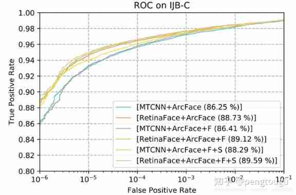
Pictured 9 Shown in FAR=1e-6 when IJB-C In the data ROC curve . We used two tricks( The samples in the image test and face detection score de weighting template ) To improve the accuracy of face authentication . Use retinaface Instead of mtcnn,TAR from 88.29% Promoted to 89.59%. This means (1) Face detection and alignment have a great impact on face recognition (2)Retinaface comparison MTCNN More powerful .
4.8 inference efficiency
At testing time ,retianface Flexible and efficient face location . Except for models with more weights (ResNet-152,262M,AP=91.8%(hard)), We also developed a lightweight model (MobileNet-0.25,1M,AP=78.2%(hard)) To speed up prediction .
For lightweight networks , We can pass a step of 4,7x7 Convolution of , Quickly reduce data size , stay P3,P4,P5 Add dense after anchors, And delete the deformation layer . Besides , The first two convolution layers are used imagenet After pre training initialization, it is fixed during retraining to obtain higher accuracy .
form 5 The time consumption of the two models with different input sizes is shown . among , The time of dense regression branches is not counted . Use TVM To accelerate model prediction , The test platform is NVIDIA Tesla P40 GPU,Intel i7-6700k cpu and ARM-RK3399.

Reference resources
【1】 K. He, G. Gkioxari, P. Dollar, and R. Girshick. Mask r-cnn. In ICCV, 2017.
【2】 J. Wang, Y. Yuan, and G. Yu. Face attention network: an effective face detector for the occluded faces. arXiv:1711.07246, 2017.
【3】 Y. Zhou, J. Deng, I. Kotsia, and S. Zafeiriou. Dense 3d face decoding over 2500fps: Joint texture and shape convolutional mesh decoders. In arxiv, 2019.
【4】 S. Zhang, R. Zhu, X. Wang, H. Shi, T. Fu, S. Wang, and T. Mei. Improved selective refinement network for face detection. arXiv:1901.06651, 2019.
【5】 VGA The resolution of the : Image size 640x480 // HD Images :1920x1080 // 4K Images :4096x2160
【6】 J. Dai, H. Qi, Y. Xiong, Y. Li, G. Zhang, H. Hu, and Y. Wei. Deformable convolutional networks. In ICCV, 2017
【7】 A. Shrivastava, A. Gupta, and R. Girshick. Training regionbased object detectors with online hard example mining. In CVPR, 2016.
Two 、pytorch_retinaface Version run library test
retinaface What's the effect , It can only be verified through comparative experiments . Here to pytorch_retinaface Version tested , This version is among all versions of the community star The highest Edition .
Data set preparation
This address contains clean Wideface Data sets :https://github.com/Linzaer/Ultra-Light-Fast-Generic-Face-Detector-1MB
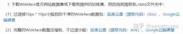
The downloaded data set contains these three :

At this time, there are only pictures in the folder , However, the data format required by the author is :

So we also lack the index file of data , At this time, use the script provided by the author wider_val.py, Export the picture information into txt file :
# -*- coding: UTF-8 -*-
'''
@author: mengting gu
@contact: [email protected]
@time: 2020/11/2  In the morning 11:47
@file: widerValFile.py
@desc:
'''
import os
import argparse

parser = argparse.ArgumentParser(description='Retinaface')
parser.add_argument('--dataset_folder', default=r'E:\pytorch\Retinaface\data\widerface\WIDER_val\images/', type=str, help='dataset path')
args = parser.parse_args()

if __name__ == '__main__':
    # testing dataset
    testset_folder = args.dataset_folder
    testset_list = args.dataset_folder[:-7] + "label.txt"

    with open(testset_list, 'r') as fr:
        test_dataset = fr.read().split()
    num_images = len(test_dataset)

    for i, img_name in enumerate(test_dataset):
        print("line i :{}".format(i))
        if img_name.endswith('.jpg'):
            print("     img_name :{}".format(img_name))
            f = open(args.dataset_folder[:-7] + 'wider_val.txt', 'a')
            f.write(img_name + '\n')
    f.close()
The complete format after export is as follows :

Each data set has a txt file
txt The content of the document is roughly like this ( With train.txt For example ), Contains image information and face location information :
# 0--Parade/0_Parade_marchingband_1_849.jpg
449 330 122 149 488.906 373.643 0.0 542.089 376.442 0.0 515.031 412.83 0.0 485.174 425.893 0.0 538.357 431.491 0.0 0.82
# 0--Parade/0_Parade_Parade_0_904.jpg
361 98 263 339 424.143 251.656 0.0 547.134 232.571 0.0 494.121 325.875 0.0 453.83 368.286 0.0 561.978 342.839 0.0 0.89
model training
python train.py --network mobile0.25
If necessary , Please download the pre training model first , Put it in weights In the folder . If you want to train from scratch , It's in data/config.py The document specifies 'pretrain': False,
Model to evaluate
mobile0.25
cd ./widerface_evaluate
python setup.py build_ext --inplace
python test_widerface.py --trained_model ./weights/mobilenet0.25_Final.pth --network mobile0.25
python widerface_evaluate/evaluation.py
After executing the second statement, it will compile .so file , Best in linux Perform all operations on the system :

After the third sentence , The model will test the data in batches :

Finish the third sentence , The assessment results are as follows :
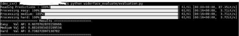
The experimental results given by the author :

3、 ... and 、GhostNet and MobileNetv3 Transplant skeleton
3.1 pytorch_retinaface Source code modification
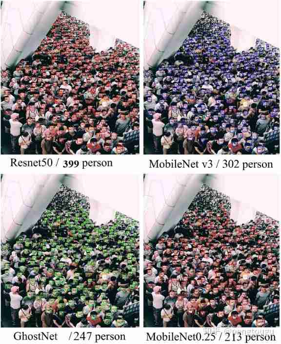
After the test in the previous section , Another image containing only one face is taken for detection , You can find ,resnet50 It takes a long time to detect a single image with only a single face , If the project pays attention to real-time mb0.25 It's a better choice , But for scenes with dense faces and small scales, it is more difficult .
If the skeleton is replaced by another network , Whether it can give consideration to real-time and accuracy ?
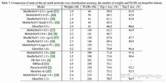
The skeleton replacement here is temporarily used ghostnet and mobilev3 The Internet ( I also want to test whether the effect of these two networks can be as outstanding as the paper ).
We are config.py Add the relevant parameter information of these two networks in the document :
cfg_gnet = {
    'name': 'ghostnet',
    'min_sizes': [[16, 32], [64, 128], [256, 512]],
    'steps': [8, 16, 32],
    'variance': [0.1, 0.2],
    'clip': True,
    'loc_weight': 2.0,
    'gpu_train': True,
    'batch_size': 16,
    'ngpu': 1,
    'epoch': 300,
    'decay1': 190,
    'decay2': 220,
    'image_size': 640,
    'pretrain': False,
    'return_layers': {'blocks1': 1, 'blocks2': 2, 'blocks3': 3},
    'in_channel': 32,
    'out_channel': 64
}
cfg_mnetv3 = {
    'name': 'mobilev3',
    'min_sizes': [[16, 32], [64, 128], [256, 512]],
    'steps': [8, 16, 32],
    'variance': [0.1, 0.2],
    'clip': True,
    'loc_weight': 2.0,
    'gpu_train': True,
    'batch_size': 16,
    'ngpu': 1,
    'epoch': 350,
    'decay1': 190,
    'decay2': 220,
    'image_size': 680,
    'pretrain': False,
    'return_layers': {'bneck1': 1, 'bneck2': 2, 'bneck3': 3},
    'in_channel': 32,
    'out_channel': 64
}
We are retinaface.py The parent class of the file specifies the relevant reference , And in IntermediateLayerGetter(backbone, cfg[‘return_layers’]) Specify the network layer to call ID, The ID stay config.py It has been indicated in the document :
def __init__(self, cfg=None, phase='train'):
    """
    :param cfg:  Network related settings.
    :param phase: train or test.
    """
    super(RetinaFace, self).__init__()
    self.phase = phase
    backbone = None
    if cfg['name'] == 'mobilenet0.25':
        backbone = MobileNetV1()
        if cfg['pretrain']:
            checkpoint = torch.load("./weights/mobilenetV1X0.25_pretrain.tar", map_location=torch.device('cpu'))
            from collections import OrderedDict
            new_state_dict = OrderedDict()
            for k, v in checkpoint['state_dict'].items():
                name = k[7:]  # remove module.
                new_state_dict[name] = v
            # load params
            backbone.load_state_dict(new_state_dict)
    elif cfg['name'] == 'Resnet50':
        import torchvision.models as models
        backbone = models.resnet50(pretrained=cfg['pretrain'])
    elif cfg['name'] == 'ghostnet':
        backbone = ghostnet()
    elif cfg['name'] == 'mobilev3':
        backbone = MobileNetV3()

    self.body = _utils.IntermediateLayerGetter(backbone, cfg['return_layers'])
We specify FPN Number of network channels , And for the three layers formulated in the model FPN The structure is fixed on each floor in_channels:
in_channels_stage2 = cfg['in_channel']
        in_channels_list = [
            in_channels_stage2 * 2,
            in_channels_stage2 * 4,
            in_channels_stage2 * 8,
        ]
        out_channels = cfg['out_channel']
        # self.FPN = FPN(in_channels_list, out_channels)
        self.FPN = FPN(in_channels_list, out_channels)
With mobile0.25 For example , From the bottom up in_channels Respectively 64,128,256( stay config.py Initial definition 'in_channel': 32, , respectively, *2,*4,*8 By analogy )
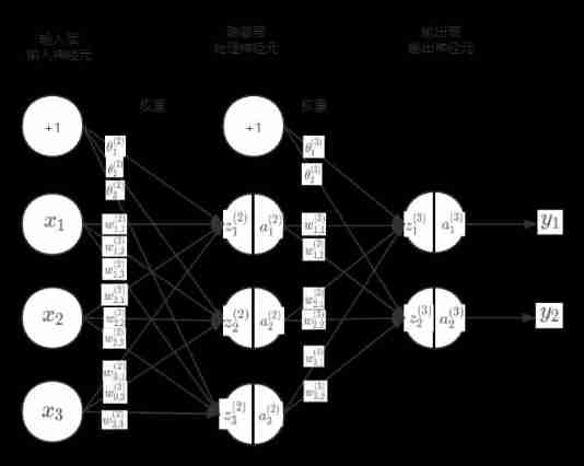
As the paper says ,pytorch The version defines SSH The three-tier structure of , And will FPN The results of the iteration are encapsulated into three groups Tensor, Respectively substitute into the calculation . Get three groups features, And then merge into a large group .
	"""
	retinaface.py → line 91 - line 97
	"""
    self.ssh1 = SSH(out_channels, out_channels)
    self.ssh2 = SSH(out_channels, out_channels)
    self.ssh3 = SSH(out_channels, out_channels)

    self.ClassHead = self._make_class_head(fpn_num=3, inchannels=cfg['out_channel'])
    self.BboxHead = self._make_bbox_head(fpn_num=3, inchannels=cfg['out_channel'])
    self.LandmarkHead = self._make_landmark_head(fpn_num=3, inchannels=cfg['out_channel'])

	"""
	retinaface.py → line 123 - line 133
	"""
	fpn = self.FPN(out)

    # SSH
    feature1 = self.ssh1(fpn[0])
    feature2 = self.ssh2(fpn[1])
    feature3 = self.ssh3(fpn[2])
    features = [feature1, feature2, feature3]

    bbox_regressions = torch.cat([self.BboxHead[i](feature) for i, feature in enumerate(features)], dim=1)
    classifications = torch.cat([self.ClassHead[i](feature) for i, feature in enumerate(features)], dim=1)
    ldm_regressions = torch.cat([self.LandmarkHead[i](feature) for i, feature in enumerate(features)], dim=1)
We are models/ghostnet.py Insert ghontnet The Internet , The network structure comes from the open source address of Noah's Ark Laboratory https://github.com/huawei-noah/ghostnet:
Classification effect comparison :
Because it contains residual convolution separation module and SE modular , The source code is relatively long , The revised network source code is as follows :
class GhostNet(nn.Module):
    def __init__(self, cfgs, num_classes=1000, width=1.0, dropout=0.2):
        super(GhostNet, self).__init__()
        # setting of inverted residual blocks
        self.cfgs = cfgs
        self.dropout = dropout

        # building first layer
        output_channel = _make_divisible(16 * width, 4)
        self.conv_stem = nn.Conv2d(3, output_channel, 3, 2, 1, bias=False)
        self.bn1 = nn.BatchNorm2d(output_channel)
        self.act1 = nn.ReLU(inplace=True)
        input_channel = output_channel

        # building inverted residual blocks
        stages = []
        block = GhostBottleneck
        for cfg in self.cfgs:
            layers = []
            for k, exp_size, c, se_ratio, s in cfg:
                output_channel = _make_divisible(c * width, 4)
                hidden_channel = _make_divisible(exp_size * width, 4)
                layers.append(block(input_channel, hidden_channel, output_channel, k, s,
                                    se_ratio=se_ratio))
                input_channel = output_channel
            # print(output_channel)
            stages.append(nn.Sequential(*layers))

        # print(len(stages))
        # output_channel = _make_divisible(exp_size * width, 4)
        # stages.append(nn.Sequential(ConvBnAct(input_channel, output_channel, 1)))
        # input_channel = output_channel

        # self.blocks = nn.Sequential(*stages)
		#  The first layer is encapsulated here block, Corresponding to config.py In file
        self.blocks1 = nn.Sequential(
            stages[0],
            stages[1],
            stages[2],
            stages[3],
            stages[4],
        )
        #  The second layer is encapsulated here block, Corresponding to config.py In file
        self.blocks2 = nn.Sequential(
            stages[5],
            stages[6],
        )
        #  Package the third layer here block, Corresponding to config.py In file
        self.blocks3 = nn.Sequential(
            stages[7],
            stages[8],
        )

        # building last several layers
        output_channel = 256
        self.global_pool = nn.AdaptiveAvgPool2d((1, 1))
        self.conv_head = nn.Conv2d(input_channel, output_channel, 1, 1, 0, bias=True)
        self.act2 = nn.ReLU(inplace=True)
        self.classifier = nn.Linear(output_channel, num_classes)

	#  The network architecture is repackaged , The pre reasoning part changes with the response
    def forward(self, x):
        x = self.conv_stem(x)
        x = self.bn1(x)
        x = self.act1(x)
        x = self.blocks1(x)
        x = self.blocks2(x)
        x = self.blocks3(x)
        # x = self.blocks(x)
        x = self.global_pool(x)
        x = self.conv_head(x)
        x = self.act2(x)
        x = x.view(x.size(0), -1)
        if self.dropout > 0.:
            x = F.dropout(x, p=self.dropout, training=self.training)
        x = self.classifier(x)
        return x
We are models/mobilev3.py Insert MobileNetv3 The Internet , The network structure comes from github Reproduced by netizens pytorch edition , True plug and play !https://github.com/kuan-wang/pytorch-mobilenet-v3:
Classification effect :

The revised source code is as follows :
#!/usr/bin/env python
# coding:utf-8
"""
Name : mobilenetv3.py
Author  : @ Chenxr
Create on   : 2021/5/8 22:45
Desc: None

class MobileNetV3(nn.Module):
    def __init__(self, num_classes=1000):
        super(MobileNetV3, self).__init__()
        self.conv1 = nn.Conv2d(3, 16, kernel_size=3, stride=2, padding=1, bias=False)
        self.bn1 = nn.BatchNorm2d(16)
        self.hs1 = hswish()


        self.bneck1 = nn.Sequential(
            Block(3, 16, 16, 16, nn.ReLU(inplace=True), None, 1),
            Block(3, 16, 64, 32, nn.ReLU(inplace=True), None, 2),
            Block(3, 32, 72, 32, nn.ReLU(inplace=True), None, 1),
            Block(5, 32, 72, 64, nn.ReLU(inplace=True), SeModule(64), 2),
            Block(5, 64, 120, 64, nn.ReLU(inplace=True), SeModule(64), 1),
            Block(5, 64, 120, 64, nn.ReLU(inplace=True), SeModule(64), 1),
        )
        self.bneck2 = nn.Sequential(
            Block(3, 64, 240, 80, hswish(), None, 2),
            Block(3, 80, 200, 80, hswish(), None, 1),
            Block(3, 80, 184, 80, hswish(), None, 1),
            Block(3, 80, 184, 128, hswish(), None, 1),
        )
        self.bneck3 = nn.Sequential(
            Block(3, 128, 480, 128, hswish(), SeModule(128), 1),
            Block(3, 128, 672, 128, hswish(), SeModule(128), 1),
            Block(5, 128, 672, 256, hswish(), SeModule(256), 1),
            Block(5, 256, 672, 256, hswish(), SeModule(256), 2),
            Block(5, 256, 960, 256, hswish(), SeModule(256), 1),
        )


        self.conv2 = nn.Conv2d(256, 960, kernel_size=1, stride=1, padding=0, bias=False)
        self.bn2 = nn.BatchNorm2d(960)
        self.hs2 = hswish()
        self.linear3 = nn.Linear(960, 1280)
        self.bn3 = nn.BatchNorm1d(1280)
        self.hs3 = hswish()
        self.linear4 = nn.Linear(1280, num_classes)
        self.init_params()
stay train.py in , We will import the embedded network , And specify the relevant configuration ( stay detect.py The same processing in the file ):
from models.retinaface import RetinaFace

parser = argparse.ArgumentParser(description='Retinaface Training')
parser.add_argument('--training_dataset', default='./data/widerface/train/label.txt', help='Training dataset directory')
parser.add_argument('--network', default='ghostnet', help='Backbone network mobile0.25 & resnet50 & ghostnet & mobilev3')
parser.add_argument('--num_workers', default=4, type=int, help='Number of workers used in dataloading')
parser.add_argument('--lr', '--learning-rate', default=0.01, type=float, help='initial learning rate')
parser.add_argument('--momentum', default=0.9, type=float, help='momentum')
parser.add_argument('--resume_net', default=None, help='resume net for retraining')
parser.add_argument('--resume_epoch', default=0, type=int, help='resume iter for retraining')
parser.add_argument('--weight_decay', default=5e-4, type=float, help='Weight decay for SGD')
parser.add_argument('--gamma', default=0.1, type=float, help='Gamma update for SGD')
parser.add_argument('--save_folder', default='./mobilev3/', help='Location to save checkpoint models')

if args.network == "mobile0.25":
    from models.retinaface_m import RetinaFace
    cfg = cfg_mnet
elif args.network == "resnet50":
    from models.retinaface_m import RetinaFace
    cfg = cfg_re50
elif args.network == "ghostnet":
    from models.retinaface_g import RetinaFace
    cfg = cfg_gnet
elif args.network == "mobilev3":
    from models.retinaface_g import RetinaFace
    cfg = cfg_mnetv3
3.2 model training
Carry out orders :nohup python train.py --network ghostnet > ghostnet.log 2>&1 & Start training
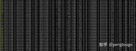
Count each network training individual epoch Duration :
- resnet50>>mobilenetv3>ghostnet-m>ghostnet-s>mobilenet0.25
3.3 Model testing and evaluation
The specific steps of evaluation have been described in the previous section , I don't want to talk about it here
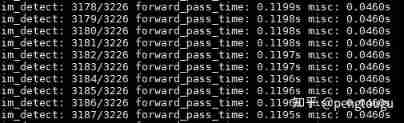
test ghostnet(se-ratio=0.25):

It can be seen that , One copy batch The test of is about 56ms about
assessment ghostnet(se-ratio=0.25):

It can be seen that ,ghostnet The recognition of small sample data and face occlusion is relatively poor .
test MobileNetV3(se-ratio=1):
It can be seen that , One copy batch The test of is about 120ms about
assessment MobileNetV3(se-ratio=1):

( The comparison here is actually a little unscientific , Because it's for use mbv3 Of se_ratio Full open benchmarking ghostnet Of se_ratio open 1/4, but ghostnet Of se_ratio Full opening will cause the model memory to soar (se-ratio=0 when weights=6M,se-ratio=0.25 when weights=12M,se-ratio=1 when weights=30M, And the accuracy barely exceeds se-ratio=1 Of MobileNetV3, Personally, I feel that the cost performance is too low ))
3.4 resnet & mbv3 & gnet & mb0.25 Contrast test
Reasoning performance comparison :
| Backbone | Computing backend | size(MB) | Framework | input_size | Run time |
|---|---|---|---|---|---|
| resnet50 | Core i5-4210M | 106 | torch | 640 | 1571 ms |
| G h o s t N e t − m S e = 0.25 GhostNet-m^{Se=0.25} GhostNet−mSe=0.25 | Core i5-4210M | 12 | torch | 640 | 403 ms |
| MobileNet v3 | Core i5-4210M | 8 | torch | 640 | 576 ms |
| MobileNet0.25 | Core i5-4210M | 1.7 | torch | 640 | 187 ms |
| MobileNet0.25 | Core i5-4210M | 1.7 | onnxruntime | 640 | 73 ms |
It can be seen that ,resnet Reasoning takes the longest , And the model memory is the largest ( But the effect is definitely the best ),mb0.25 Take the least time , But the accuracy is the lowest , but gnet and mbv3 In the above model, it is more compatible with real-time and accuracy , You can try to gpu Next run , There will be unexpected gains ~
Test performance comparison :
| Backbone | Easy | Medium | Hard |
|---|---|---|---|
| resnet50 | 95.48% | 94.04% | 84.43% |
| MobileNet v3 S e = 1 ^{Se=1} Se=1 | 93.48% | 91.23% | 80.19% |
| G h o s t N e t − m S e = 0.25 GhostNet-m^{Se=0.25} GhostNet−mSe=0.25 | 93.35% | 90.84% | 76.11% |
| MobileNet0.25 | 90.70% | 88.16% | 73.82% |
Single picture test effect comparison :
Add :
- Single frame of the test Infer Time= Reason for a minute / Number of frames processed in this minute
- In fact, it doesn't need to be so high in actual production input_size( Main survey 2-3m Detection performance in )
- The above tests are CPU Proceed under , And the author's notebook has been standby 6 Over the year , It is about to reach the end of its life ( The computer was repaired yesterday ... A bad day )
- Personal computers are different , The tested performance may deviate , But it should not be big
summary :
- For business scenarios with a single background , Seems to pay more attention to real-time , Personally, I prefer mb0.25 Version and ghostnet edition
- 5 month 10 In the future , The passing team proposed a stronger and more superior face detection framework , You can refer to my other blogs to understand Later, I will contribute onnxruntime Call the script of the model
- The code is open source , Welcome white whoring and star:
github.com/pengtougu/Retinaface_Ghost
thank
thank Sansa shi The boss has a solid foundation in literature study , To present such a perfect thesis study report , Very profitable
thank biubug6 The boss is excellent pytorch Duplicate version , So that the author can build his own roof truss on a building
There are many graduate leaders and bigwigs from all walks of life ~
边栏推荐
- Height of life
- Thread deadlock -- conditions for deadlock generation
- Introduction à l'outil nmap et aux commandes communes
- LeetCode精选200道--链表篇
- 分布式定时任务之XXL-JOB
- "Hands on learning in depth" Chapter 2 - preparatory knowledge_ 2.1 data operation_ Learning thinking and exercise answers
- leetcode 865. Smallest Subtree with all the Deepest Nodes | 865. The smallest subtree with all the deepest nodes (BFs of the tree, parent reverse index map)
- Semantic segmentation | learning record (4) expansion convolution (void convolution)
- Random walk reasoning and learning in large-scale knowledge base
- Leetcode question brushing record | 283_ Move zero
猜你喜欢
Ml backward propagation
![[knowledge atlas paper] minerva: use reinforcement learning to infer paths in the knowledge base](/img/cb/2cc490c11d88841e39c8b42dd88189.jpg)
[knowledge atlas paper] minerva: use reinforcement learning to infer paths in the knowledge base

Master go game through deep neural network and tree search

Popular science | what is soul binding token SBT? What is the value?

C language -cmake cmakelists Txt tutorial
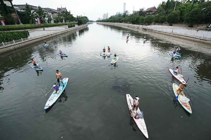
Strive to ensure that domestic events should be held as much as possible, and the State General Administration of sports has made it clear that offline sports events should be resumed safely and order
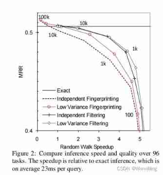
Random walk reasoning and learning in large-scale knowledge base
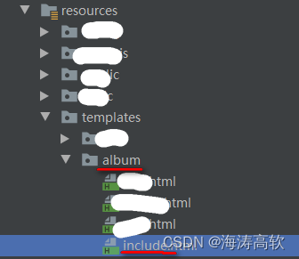
th:include的使用

Gaussian filtering and bilateral filtering principle, matlab implementation and result comparison
![[knowledge map paper] Devine: a generative anti imitation learning framework for knowledge map reasoning](/img/c1/4c147a613ba46d81c6805cdfd13901.jpg)
[knowledge map paper] Devine: a generative anti imitation learning framework for knowledge map reasoning
随机推荐
如何用Diffusion models做interpolation插值任务?——原理解析和代码实战
阿南的判断
Talk about the realization of authority control and transaction record function of SAP system
很多小伙伴不太了解ORM框架的底层原理,这不,冰河带你10分钟手撸一个极简版ORM框架(赶快收藏吧)
Is it necessary for project managers to take NPDP? I'll tell you the answer
Industrial Development and technological realization of vr/ar
The circuit is shown in the figure, r1=2k Ω, r2=2k Ω, r3=4k Ω, rf=4k Ω. Find the expression of the relationship between output and input.
Applet running under the framework of fluent 3.0
Key points of data link layer and network layer protocol
What are the types of system tests? Let me introduce them to you
Height of life
Ml backward propagation
XMeter Newsletter 2022-06|企业版 v3.2.3 发布,错误日志与测试报告图表优化
Completion report of communication software development and Application
Literature reading and writing
VR/AR 的产业发展与技术实现
Introduction to grpc for cloud native application development
Ml self realization / logistic regression / binary classification
魚和蝦走的路
阿锅鱼的大度