当前位置:网站首页>Beam pattern analysis based on spectral weighting
Beam pattern analysis based on spectral weighting
2022-06-10 18:56:00 【Master World】
Beam pattern analysis based on spectral weighting
Spectral weighting
This article mainly analyzes the linear array , The following formula gives u u u The derivation formula of spatial beam pattern
B u ( u ) = ω H v u ( u ) = e − j N − 1 2 2 π d λ u ∑ n = 0 N − 1 ω n ∗ e j n 2 π d λ u B_u(u)=\omega^Hv_u(u)=e^{-j\frac{N-1}{2}\frac{2\pi d}{\lambda}u}\sum_{n=0}^{N-1}\omega^*_ne^{jn\frac{2\pi d}{\lambda}u} Bu(u)=ωHvu(u)=e−j2N−1λ2πdun=0∑N−1ωn∗ejnλ2πdu
We can see , The beam pattern is the product of weight and manifold vector , This paper mainly analyzes the different effects of different weights on the beam pattern , Because the weights considered below are all real symmetric , So you can put n The positions of the array elements are replaced by the following labels n ~ = n − N − 1 2 , n = 0 , 1 , ⋯ , N − 1 \tilde{n}=n-\frac{N-1}{2},n=0,1,\cdots,N-1 n~=n−2N−1,n=0,1,⋯,N−1
cosine weighting
consider N In the case of an odd number ,cosine A weight of ω ( n ~ ) = s i n ( π 2 N ) c o s ( π n ~ N ) , − N − 1 2 ≤ n ~ ≤ N − 1 2 \omega(\tilde{n})=sin(\frac{\pi}{2N})cos(\pi\frac{\tilde{n}}{N}),-\frac{N-1}{2}\leq \tilde{n}\leq\frac{N-1}{2} ω(n~)=sin(2Nπ)cos(πNn~),−2N−1≤n~≤2N−1
among s i n ( π 2 N ) sin(\frac{\pi}{2N}) sin(2Nπ) It's a constant , The purpose is to yes B u ( 0 ) = 1 , hold c o s i n e Write become finger Count shape type , By Step change shape most end can With have to To B_u(0)=1, hold cosine In exponential form , Step by step deformation will eventually lead to Bu(0)=1, hold cosine Write become finger Count shape type , By Step change shape most end can With have to To
B u ( u ) = 1 2 s i n ( π 2 N ) { s i n ( N π 2 ( u − 1 N ) ) s i n ( π 2 ( u − 1 N ) ) + s i n ( N π 2 ( u + 1 N ) ) s i n ( π 2 ( u + 1 N ) ) } B_u(u)=\frac{1}{2}sin(\frac{\pi}{2N})\{\frac{sin(\frac{N\pi}{2}(u-\frac{1}{N}))}{sin(\frac{\pi}{2}(u-\frac{1}{N}))}+\frac{sin(\frac{N\pi}{2}(u+\frac{1}{N}))}{sin(\frac{\pi}{2}(u+\frac{1}{N}))}\} Bu(u)=21sin(2Nπ){ sin(2π(u−N1))sin(2Nπ(u−N1))+sin(2π(u+N1))sin(2Nπ(u+N1))}
We can make direct use of the computing power of the computer , Let it help us deal with the product of weights and manifold vectors , The results are given below 
We can see that the side lobe becomes lower , And the main lobe widened , Let's take a look at the comparison of various data 
matlab Code
clear all
close all

M=11;
d=0.5;              % sensor spacing wrt wavelength
D = [-(M-1)/2:1:(M-1)/2]*d; % sensor positions in wavelengths
% weights, normalized so that w(0)=1
W_unf = ones(1,M);
W_cos = cos(pi*D*2/M);

% Beampatterns
u = [0:0.001:1];
A = exp(-j*2*pi*D.'*u);
G_unf = W_unf*A;
G_unf = G_unf/(max(abs(G_unf)));
G_cos = W_cos*A;
G_cos = G_cos/(max(abs(G_cos)));
figure
% array only
clf
plot(u,20*log10(abs(G_unf)),'--')
hold on
plot(u,20*log10(abs(G_cos)),'-')
hold off
axis([0 1 -80 0])
%title([int2str(M) ' element array'])
h=legend('Uniform','Cosine');
set(h,'Fontsize',12)
xlabel('\it u','Fontsize',14)
ylabel('Beam pattern (dB)','Fontsize',14)
Raised cosine weighting
A weight ω ( n ~ ) = c ( p ) ( p + ( 1 − p ) c o s ( π n ~ N ) ) , n ~ = − N − 1 2 , ⋯ , N − 1 2 \omega(\tilde n)=c(p)(p+(1-p)cos(\pi\frac{\tilde n}{N})),\tilde n =-\frac{N-1}{2}, \cdots,\frac{N-1}{2} ω(n~)=c(p)(p+(1−p)cos(πNn~)),n~=−2N−1,⋯,2N−1
among c ( p ) c(p) c(p) It's a constant , bring B u ( 0 ) = 1 B_u(0)=1 Bu(0)=1 c ( p ) = p N + ( 1 − p ) 2 s i n ( π 2 N ) c(p)=\frac{p}{N}+\frac{(1-p)}{2}sin(\frac{\pi}{2N}) c(p)=Np+2(1−p)sin(2Nπ)
The figure below shows p = 0.31 , 0.17 , 0 p=0.31,0.17,0 p=0.31,0.17,0 Beam pattern at 
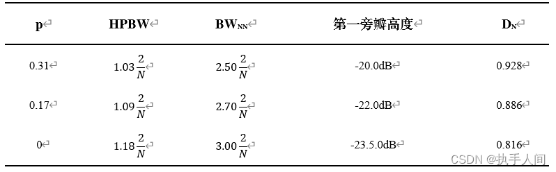
When p p p Less hours , The height of the first side lobe decreases , The main beam width increases , So we can already make HPBW Narrowing , And the first side lobe is much lower than that in the case of uniform distribution
matlab Code
clear all
close all

M=11;
d=0.5;             % sensor spacing wrt wavelength
D = [-(M-1)/2:1:(M-1)/2]*d; % sensor positions in wavelengths

% weights, normalized so that w(0)=1
p=[0;0.17;0.31;1];
W_rcos = p*ones(1,M)+(ones(4,1)-p)*cos(pi*D*2/M);

% Beampatterns
u = [0:0.001:1];
c=p+(ones(4,1)-p)*2/pi;
A = exp(-j*2*pi*D.'*u);
G_rcos = W_rcos*A;
for m=1:4
 G_rcos(m,:) = G_rcos(m,:)/(max(abs(G_rcos(m,:))));
end

figure
clf
plot(u,20*log10(abs(G_rcos(3,:))),'-.')
hold on
plot(u,20*log10(abs(G_rcos(2,:))),'--')
plot(u,20*log10(abs(G_rcos(1,:))),'-')
hold off
axis([0 1 -80 0])
h=legend('{\it p}=0.31','{\it p}=0.17','{\it p}=0');
set(h,'Fontsize',12)
xlabel('\it u','Fontsize',14)
ylabel('Beam pattern (dB)','Fontsize',14)
cosinem weighting
A series of cosine weighting , formation c o s m ( π n ~ N ) cos^m(\frac{\pi\tilde n}{N}) cosm(Nπn~),z The weight of the array is
ω m ( n ~ ) = { c 2 c o s 2 ( π n ~ N ) , m = 2 c 3 c o s 3 ( π n ~ N ) , m = 3 c 4 c o s 4 ( π n ~ N ) , m = 4 \omega_m(\tilde n) = \begin{cases} c_2cos^2(\frac{\pi\tilde n}{N}), & m=2 \\ c_3cos^3(\frac{\pi\tilde n}{N}), & m=3 \\ c_4cos^4(\frac{\pi\tilde n}{N}),& m=4 \\ \end{cases} ωm(n~)=⎩⎪⎨⎪⎧c2cos2(Nπn~),c3cos3(Nπn~),c4cos4(Nπn~),m=2m=3m=4
among c 2 , c 3 , c 4 c_2,c_3,c_4 c2,c3,c4 It is still a normalized constant
The following figure shows the beam pattern , When m increases , Sidelobe reduction , But the main beam becomes wider 

matlab Code
clear all
close all

M=11;
d=0.5;                        % sensor spacing wrt wavelength
D = [-(M-1)/2:1:(M-1)/2]*d;   % sensor positions in wavelengths

% weights, normalized so that w(0)=1
W_cos2 = cos(pi*D*2/M).^2;
W_cos3 = cos(pi*D*2/M).^3;
W_cos4 = cos(pi*D*2/M).^4;

% Beampatterns

u = [0:0.001:1];
A = exp(-j*2*pi*D.'*u);
G_cos2 = W_cos2*A;
G_cos2 = G_cos2/(max(abs(G_cos2)));
G_cos3 = W_cos3*A;
G_cos3 = G_cos3/(max(abs(G_cos3)));
G_cos4 = W_cos4*A;
G_cos4 = G_cos4/(max(abs(G_cos4)));

figure
clf
plot(u,20*log10(abs(G_cos2)),'--')
hold on
plot(u,20*log10(abs(G_cos3)),'-')
plot(u,20*log10(abs(G_cos4)),'-.')
hold off
axis([0 1 -80 0])
h=legend('{\it m}=2','{\it m}=3','{\it m}=4');
set(h,'Fontsize',12)
xlabel('\it u','Fontsize',14)
ylabel('Beam pattern (dB)','Fontsize',14)
summary
The above analysis cosine Weighting and its several deformations , Overall speaking ,cosine Weighting widens the width of the main lobe but lowers the height of the first side lobe , And in the raised cosine weighting ,p The smaller the size, the more obvious the trend , Also in cosine Of m Power weighted ,m The bigger, the more obvious .
边栏推荐
猜你喜欢

元数据管理,数字化时代企业的基础建设

The value of Bi in the enterprise: business analysis and development decision

How to transform digital transformation? Which way?

Seata安装Window环境

Adobe Premiere foundation - tool use (selection tool, razor tool, and other common tools) (III)
Metadata management, the basic construction of enterprises in the digital era
干货 | 一文搞定 uiautomator2 自动化测试工具使用
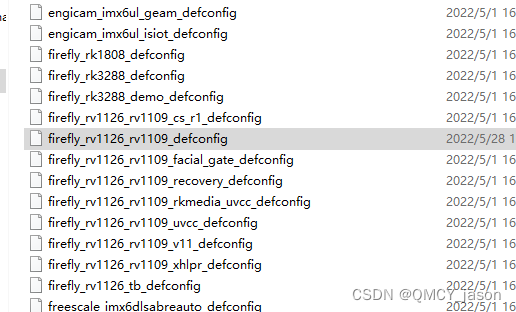
RK1126 新添加一个模块
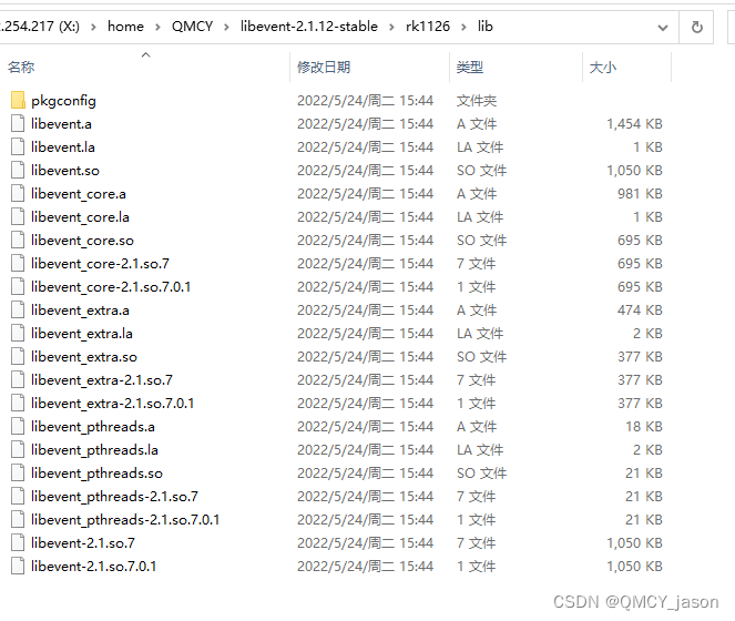
瑞芯微RK1126平台 平台移植libevent 交叉编译libevent

第一章 SQL操作符
随机推荐
实时商业智能BI(二):合理的ETL架构设计实现准实时商业智能BI
Screen output of DB2 stored procedure, output parameters, and return result set
数据治理经典6大痛点?这本书教你解决
Stream生成的3张方式-Lambda
直播预告 | 社交新纪元,共探元宇宙社交新体验
vcsa7u3c安装教程
[kuangbin]专题十二 基础DP1
商业智能BI的服务对象,企业管理者的管理“欲望”该如何实现?
Form form of the uniapp uview framework, input the verification mobile number and verification micro signal
不确定性推理:让模型知道自己不知道
Salesmartly | add a new channel slack to help you close the customer relationship
Adobe Premiere foundation - material nesting (animation of Tiktok ending avatar) (IX)
Db2 SQL PL的动态SQL
Wireshark学习笔记(一)常用功能案例和技巧
数字化时代,企业如何进行数据安全治理,保障数据资产安全
Adobe Premiere Basic - tool use (select tools, rasoir tools, and other Common Tools) (III)
Adobe Premiere基础(动画制作)(七)
Opencv does not rely on any third-party database for face detection
[QNX hypervisor 2.2 user manual] 3.3 configure guest
In 2021, the world's top ten analog IC suppliers: Ti ranked first, and skyworks' revenue growth was the highest