当前位置:网站首页>30 minutes to understand PCA principal component analysis
30 minutes to understand PCA principal component analysis
2022-07-06 18:13:00 【The way of Python data】
source : Algorithm food house
This article shares with you PCA The concept of principal component analysis and in Python The use of . I also shared two articles before , It's also very good , It can be combined to see , Deepen the understanding .
Article to read PCA The mathematical principle of the algorithm
Let's talk about the dimensionality reduction algorithm :PCA Principal component analysis
PCA Principal component analysis algorithm (Principal Components Analysis) It is one of the most commonly used dimensionality reduction algorithms . With low information loss ( Measured by the variance of distribution between samples ) Reduce the number of features .
PCA Algorithms can help Analyze the components with the greatest distribution difference in the sample ( The principal components ), Help data visualization ( Down to 2 Dimension or 3 After dimension, it can be visualized with scatter diagram ), Sometimes it can also play Reduce the noise in the sample The role of ( Part of the lost information is noise ).
One 、PCA Intuitive understanding of algorithms
Intuitively ,PCA Principal component analysis is similar to finding the direction long axis with the greatest difference in each position of a group of sample points in turn .
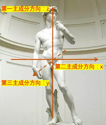
Suppose that all cells in a person are regarded as sample points one by one . These sample points can be used 3 Coordinates to represent , From left to right x Direction , From front to back y Direction , From bottom to top is z Direction .
So what is their first principal component ? The long axis corresponding to the first principal component is along the direction from the foot to the head , That is, the usual up and down direction , namely z Direction . This direction is the main long axis . The position difference of these sample points is basically 70% The above comes from the difference in this direction .
What is their second principal component ? The second principal component corresponds to the direction from left arm to right arm , That is, the usual left-right direction , namely y Direction . This direction is perpendicular to the long axis of the first principal component , The location differences of these sample points are about 20% Left and right come from the difference in this direction .
What is their third principal component ? The third principal component direction is along the direction from the chest to the back , That is, the usual fore-and-aft direction , namely x Direction . This direction is perpendicular to the long axis of the first two principal components , The position difference of sample points is generally less than 10% The difference from this direction , Of course , Except for some students who are more rounded .
Now? , If you want to reduce the coordinates of these sample points to 2 One to indicate , And keep as much information about the location differences between sample points as possible , that , obviously , The coordinates of the first principal component and the second principal component should be retained .
Now? , Suppose this person is lying on a reclining chair , Now the first principal component of these sample points is obviously no longer from bottom to top z Direction . We should rotate our coordinate system , Give Way z The axis is in the same direction as the reclining chair , This new z The direction is the first principal component direction of these sample points . Similarly , You also need to rotate x Axis and y The axis obtains the new second principal component direction and the third principal component direction .
The process of rotating the old coordinate system to find the direction of the principal component is PCA Principal component analysis .
Two 、PCA Mathematical description of the algorithm
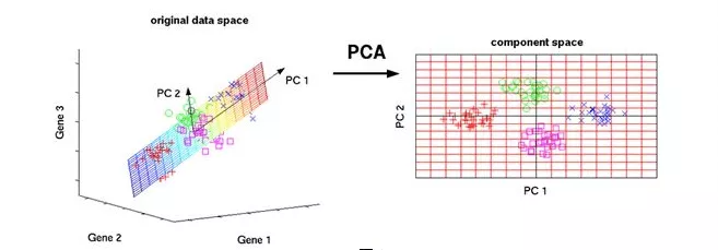
PCA Principal component analysis (Principal Components Analysis) It's a kind of passing Orthogonal linear combination The way , Maximize the variance between samples Of Dimension reduction Method .
From a geometric point of view ,PCA The principal component analysis method can be regarded as through Orthogonal transformation , Rotate and translate the coordinate system , The first several new coordinates with the largest variance of the projection coordinates of the sample points are retained .
Here are a few key words to explain :
Dimension reduction : Take the original sample m Victor requisitioned less k Features replace . Dimension reduction algorithm can be understood as a data compression method , It may lose some information .
Orthogonal linear combination :k A new feature is through m It is produced by linear combination of Gejiu features , also k The coefficient vector of a linear combination is the unit vector , And they are orthogonal to each other .
Maximize the variance between samples : The first 1 Principal component features maximize the characteristic variance between samples , The first 2 The three principal component features are satisfying the 1 Maximize the characteristic variance between samples under the orthogonal constraints of principal components ……
3、 ... and 、PCA Example of algorithm switching
In the following example, we call sklearn Medium PCA Dimension reduction algorithm interface , Dimensionality reduction of Boston house price data set (13 Dimension down to 7 dimension ).
import numpy as np
import pandas as pd

import matplotlib.pyplot as plt
from sklearn import datasets

boston = datasets.load_boston()
dfdata = pd.DataFrame(boston.data,columns = boston.feature_names)
dfdata.head()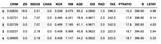
#  The value range of different features varies greatly , We first normalize the standard normal
#  The normalized result is taken as  PCA Dimension reduction input
from sklearn.preprocessing import StandardScaler
scaler = StandardScaler()
scaler.fit(dfdata.values)
X_input = scaler.transform(dfdata.values)

#  Our inputs are 506 Samples ,13 Whitman's sign
print(X_input.shape)
(506, 13)# application PCA Carry out dimension reduction
from sklearn.decomposition import PCA
pca = PCA(n_components=7)
pca.fit(X_input)
X_output = pca.transform(X_input)
# After the dimension reduction , Only 7 Whitman's sign
print(X_output.shape)(506, 7)# Check the variance corresponding to each principal component and the proportion in the total variance
# You can see before 7 Principal components have explained the distribution of samples 90% The difference .
print("explained_variance:")
print(pca.explained_variance_)
print("explained_variance_ratio:")
print(pca.explained_variance_ratio_)
print("total explained variance ratio of first 7 principal components:")
print(sum(pca.explained_variance_ratio_)explained_variance:
[6.1389812 1.43611329 1.2450773 0.85927328 0.83646904 0.65870897
0.5364162 ]
explained_variance_ratio:
[0.47129606 0.11025193 0.0955859 0.06596732 0.06421661 0.05056978
0.04118124]
total explained variance ratio of first 7 principal components:
0.8990688406240493# Visualize the variance of each principal component contribution
%matplotlib inline
%config InlineBackend.figure_format = 'svg'
import matplotlib.pyplot as plt
plt.figure()
plt.plot(np.arange(1,8),pca.explained_variance_,linewidth=2)
plt.xlabel('components_n', fontsize=16)
plt.ylabel('explained_variance_', fontsize=16)
plt.show()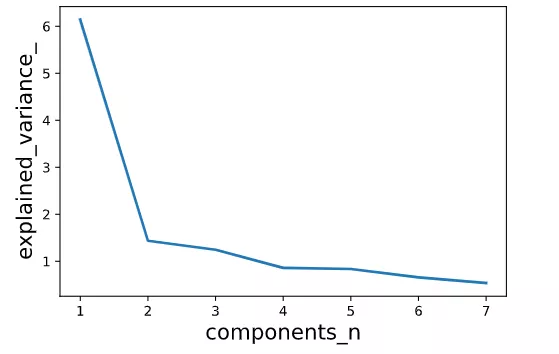
#  Check the orthogonal transformation matrix corresponding to the dimension reduction , That is, each projection vector
W = pca.components_
#  Verify orthogonality
np.round(np.dot(W,np.transpose(W)),6)
array([[ 1., 0., -0., -0., -0., 0., -0.],
[ 0., 1., -0., 0., 0., -0., -0.],
[-0., -0., 1., 0., -0., 0., -0.],
[-0., 0., 0., 1., -0., -0., 0.],
[-0., 0., -0., -0., 1., 0., 0.],
[ 0., -0., 0., -0., 0., 1., -0.],
[-0., -0., -0., 0., 0., -0., 1.]])# Visualize the first two dimensions of the reduced dimension data
%matplotlib inline
%config InlineBackend.figure_format = 'svg'
plt.scatter(X_output[:,0],X_output[:,1])
plt.xlabel("components_1")
plt.ylabel("components_2")
plt.show()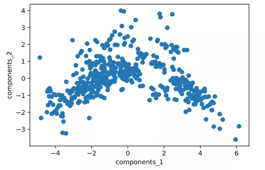
Four 、PCA The mathematical principle of the algorithm
High number reminder ahead .
Underneath PCA Deduction of mathematical principle of Algorithm , Certificate No k The principal component projection vector is exactly the... Of the covariance matrix of the sample k Eigenvectors corresponding to large eigenvalues .
The following deduction will use some knowledge of linear algebra and calculus in Advanced Mathematics .
Students without relevant mathematical foundation can skip , In practice, just master PCA Intuitive concept of the algorithm and how to use it , Basically enough .
Suppose that the characteristics of the sample are represented by a matrix , Each line represents a sample , Each column represents a feature .
Assuming that Dimensional , I.e. samples , Whitman's sign .
Now look for the first principal component .
Suppose the first principal component projection vector is , It is a unit column vector , Dimension is ,
Then the coordinate after projection is
The coordinate variance between the projected samples can be expressed as
Bars mean averaging the samples , Because it has nothing to do with the sample , It can be reduced to :
be aware It happens to be The covariance matrix of .
Next we want to maximize the coordinate variance , At the same time, the unit length constraint must be satisfied :
For extreme value conditions with constraints , We can apply Lagrange multiplier method in calculus . Construct the following Lagrange function .
402 Payment Required
The subscript representation can be used to prove , For quadratic form , There is the following vector derivation formula :
We can deduce that :
402 Payment Required
It can be seen that , Is the eigenvalue of the covariance matrix , Is the corresponding eigenvector . Because the covariance matrix is a real symmetric matrix , Its characteristic value must be greater than or equal to 0.
meanwhile , The coordinate variance between the projected samples can be expressed as :
402 Payment Required
To maximize the coordinate variance between samples , The largest eigenvalue of the covariance matrix should be taken , Then it should be the eigenvector corresponding to the maximum eigenvalue of the covariance matrix .
Similarly , It can be proved that k The first principal component projection vector is the... Of the covariance matrix k Eigenvectors corresponding to large eigenvalues .
Because the eigenvectors of different eigenvalues of the matrix are orthogonal to each other , Therefore, these projection vectors satisfy the orthogonal condition .
边栏推荐
- Distinguish between basic disk and dynamic disk RAID disk redundant array
- Jielizhi obtains the currently used dial information [chapter]
- node の SQLite
- scratch疫情隔离和核酸检测模拟 电子学会图形化编程scratch等级考试三级真题和答案解析2022年6月
- OliveTin能在网页上安全运行shell命令(上)
- Flet教程之 13 ListView最常用的滚动控件 基础入门(教程含源码)
- 偷窃他人漏洞报告变卖成副业,漏洞赏金平台出“内鬼”
- RB157-ASEMI整流桥RB157
- Interview shock 62: what are the precautions for group by?
- 传统家装有落差,VR全景家装让你体验新房落成效果
猜你喜欢
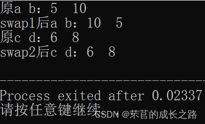
C language exchanges two numbers through pointers
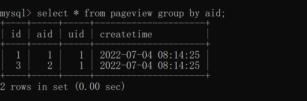
Interview assault 63: how to remove duplication in MySQL?

There is a gap in traditional home decoration. VR panoramic home decoration allows you to experience the completion effect of your new house

面向程序员的精品开源字体
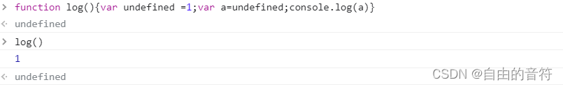
Interesting - questions about undefined

第三季百度网盘AI大赛盛夏来袭,寻找热爱AI的你!

【Swoole系列2.1】先把Swoole跑起来

Declval of template in generic programming
2019 Alibaba cluster dataset Usage Summary

虚拟机VirtualBox和Vagrant安装
随机推荐
Running the service with systemctl in the container reports an error: failed to get D-Bus connection: operation not permitted (solution)
What is the reason why the video cannot be played normally after the easycvr access device turns on the audio?
FMT open source self driving instrument | FMT middleware: a high real-time distributed log module Mlog
Alibaba brand data bank: introduction to the most complete data bank
78 岁华科教授逐梦 40 载,国产数据库达梦冲刺 IPO
Distinguish between basic disk and dynamic disk RAID disk redundant array
Easy introduction to SQL (1): addition, deletion, modification and simple query
Awk command exercise
關於這次通信故障,我想多說幾句…
Manifest of SAP ui5 framework json
scratch疫情隔离和核酸检测模拟 电子学会图形化编程scratch等级考试三级真题和答案解析2022年6月
开源与安全的“冰与火之歌”
递归的方式
Growth of operation and maintenance Xiaobai - week 7
Is it meaningful for 8-bit MCU to run RTOS?
Interview shock 62: what are the precautions for group by?
F200 - UAV equipped with domestic open source flight control system based on Model Design
Jielizhi obtains the currently used dial information [chapter]
How to solve the error "press any to exit" when deploying multiple easycvr on one server?
F200——搭载基于模型设计的国产开源飞控系统无人机