PI control of three-phase grid connected inverter - off grid mode

Off grid control of three-phase grid connected inverter

The basic difference between inverter parallel and off grid control

   When the three-phase grid connected inverter is connected to the grid , Its main function is to transmit electric energy to the large power grid . At this time, the system parallel node voltage is Big grid clamping , Therefore, it is only necessary to control the inverter to output the current that meets the power requirements , Control objectives can be achieved , Therefore, the grid connected inverter in this state is generally equivalent to Current source .

   When the three-phase grid connected inverter is off grid , Its main function is to output the voltage that meets the load operation conditions , Current system System output current All by load Self parameters decision . Therefore, the grid connected inverter in this state is generally equivalent to Voltage source .

Basic topology of off grid inverter

   The following figure shows the inverter topology in the off grid state , Here we use pure resistance instead of pure resistive load ：

   Take the direction of the inverter pointing to the load current as the positive direction of the current reference , In the picture $i_a$ The direction indicated is positive .

$$\{\begin{array}{c}{U}_a-L\frac{d{i}_a}{dt}-i_{a}R-U_{Ca}=0\\ U_b-L\frac{d{i}_b}{dt}-i_{b}R-U_{Cb}=0\\ U_c-L\frac{d{i}_c}{dt}-i_{c}R-U_{Cc}=0\\ C\frac{d{u}_{Ca}}{dt}=i_a-i_{ga}\\ C\frac{d{u}_{Cb}}{dt}=i_b-i_{gb}\\ C\frac{d{u}_{Cc}}{dt}=i_c-i_{gc}\end{array}\text{\hspace{1em}(1)}$$
   You can get ：
$$\{\begin{array}{c}\frac{d{i}_a}{dt}=\frac{1}{L}{U}_a-\frac{R}{L}{i}_a-\frac{1}{L}{U}_{Ca}\\ \frac{d{i}_b}{dt}=\frac{1}{L}{U}_b-\frac{R}{L}{i}_b-\frac{1}{L}{U}_{Cb}\\ \frac{d{i}_c}{dt}=\frac{1}{L}{U}_c-\frac{R}{L}{i}_c-\frac{1}{L}{U}_{Cc}\\ \frac{d{u}_{Ca}}{dt}=\frac{1}{C}{i}_a-\frac{1}{C}{i}_{ga}\\ \frac{d{u}_{Cb}}{dt}=\frac{1}{C}{i}_b-\frac{1}{C}{i}_{gb}\\ \frac{d{u}_{Cc}}{dt}=\frac{1}{C}{i}_c-\frac{1}{C}{i}_{gc}\end{array}\text{\hspace{1em}(2)}$$

   In the form of a matrix ：

$$\{\begin{array}{c}\left[\begin{array}{c}\frac{d{i}_a}{dt}\\ \frac{d{i}_b}{dt}\\ \frac{d{i}_c}{dt}\end{array}\right]=\frac{1}{L}\left[\begin{array}{c}{U}_a\\ U_b\\ U_c\end{array}\right]-\frac{R}{L}\left[\begin{array}{c}{i}_a\\ i_b\\ i_c\end{array}\right]-\frac{1}{L}\left[\begin{array}{c}{U}_{Ca}\\ U_{Cb}\\ U_{Cc}\end{array}\right]\\ \left[\begin{array}{c}\frac{d{U}_{Ca}}{dt}\\ \frac{d{U}_{Cb}}{dt}\\ \frac{d{U}_{Cc}}{dt}\end{array}\right]=\frac{1}{C}\left[\begin{array}{c}{i}_a\\ i_b\\ i_c\end{array}\right]-\frac{1}{C}\left[\begin{array}{c}{i}_{ga}\\ i_{gb}\\ i_{gc}\end{array}\right]\end{array}\text{\hspace{1em}(3)}$$

$\alpha \beta$ Inverter equation in coordinate system

   And the known abc-$\alpha \beta$ The positive and inverse transformation matrix is ：
$$\left[\begin{array}{c}{U}_{\alpha }\\ U_{\beta }\\ U_0\end{array}\right]=T_{abc-\alpha \beta }\left[\begin{array}{c}{U}_a\\ U_b\\ U_c\end{array}\right]=\frac{2}{3}\times \left[\begin{array}{ccc}1& -\frac{1}{2}& -\frac{1}{2}\\ 0& \frac{\sqrt{3}}{2}& -\frac{\sqrt{3}}{2}\\ 1& 1& 1\end{array}\right]\left[\begin{array}{c}{U}_a\\ U_b\\ U_c\end{array}\right]\text{\hspace{1em}(4)}$$

$$\left[\begin{array}{c}{U}_a\\ U_b\\ U_c\end{array}\right]=T_{\alpha \beta -abc}\left[\begin{array}{c}{U}_{\alpha }\\ U_{\beta }\\ U_0\end{array}\right]=\left[\begin{array}{ccc}1& 0& \frac{1}{2}\\ -\frac{1}{2}& \frac{\sqrt{3}}{2}& \frac{1}{2}\\ -\frac{1}{2}& -\frac{\sqrt{3}}{2}& \frac{1}{2}\end{array}\right]\left[\begin{array}{c}{U}_{\alpha }\\ U_{\beta }\\ U_0\end{array}\right]\text{\hspace{1em}(5)}$$

   Here we add 0 The axis is to make the transformation matrix into a square matrix , It is conducive to the inversion , actually 0 Axis No participation Control operation uses .

   fitting （3） Multiply both sides at the same time $T_{abc-\alpha \beta }$ The inverter equation can be transformed to $\alpha \beta$ In coordinate system , Available ：
$$\begin{array}{c}{T}_{abc-\alpha \beta }\left[\begin{array}{c}\frac{d{i}_a}{dt}\\ \frac{d{i}_b}{dt}\\ \frac{d{i}_c}{dt}\end{array}\right]=\frac{1}{L}{T}_{abc-\alpha \beta }\left[\begin{array}{c}{U}_a\\ U_b\\ U_c\end{array}\right]-\frac{R}{L}{T}_{abc-\alpha \beta }\left[\begin{array}{c}{i}_a\\ i_b\\ i_c\end{array}\right]-\frac{1}{L}{T}_{abc-\alpha \beta }\left[\begin{array}{c}{U}_{Ca}\\ U_{Cb}\\ U_{Cc}\end{array}\right]\end{array}$$

Note here that only
$$\left[\begin{array}{c}{U}_{\alpha }\\ U_{\beta }\\ U_0\end{array}\right]=T_{abc-\alpha \beta }\left[\begin{array}{c}{U}_a\\ U_b\\ U_c\end{array}\right]$$
therefore $T_{abc-\alpha \beta }\left[\begin{array}{c}\frac{d{i}_a}{dt}\\ \frac{d{i}_b}{dt}\\ \frac{d{i}_c}{dt}\end{array}\right]$ It needs to be calculated separately , The calculation process is as follows ：
$${\left[\begin{array}{c}{i}_{\alpha }\\ i_{\beta }\\ i_0\end{array}\right]}^{\prime }=(T_{abc-\alpha \beta }\left[\begin{array}{c}{i}_a\\ i_b\\ i_c\end{array}\right]{)}^{\prime }=(T_{abc-\alpha \beta }{)}^{\prime }\left[\begin{array}{c}{i}_a\\ i_b\\ i_c\end{array}\right]+(T_{abc-\alpha \beta })\left[\begin{array}{c}\frac{d{i}_a}{dt}\\ \frac{d{i}_b}{dt}\\ \frac{d{i}_c}{dt}\end{array}\right]$$

therefore
$$T_{abc-\alpha \beta }\left[\begin{array}{c}\frac{d{i}_a}{dt}\\ \frac{d{i}_b}{dt}\\ \frac{d{i}_c}{dt}\end{array}\right]=(T_{abc-\alpha \beta }\left[\begin{array}{c}{i}_a\\ i_b\\ i_c\end{array}\right]{)}^{\prime }-(T_{abc-\alpha \beta }{)}^{\prime }\left[\begin{array}{c}{i}_a\\ i_b\\ i_c\end{array}\right]$$
and $(T_{abc-\alpha \beta })$ Is a constant matrix , therefore
$$(T_{abc-\alpha \beta }{)}^{\prime }=0$$

therefore ：
$$T_{abc-\alpha \beta }\left[\begin{array}{c}\frac{d{i}_a}{dt}\\ \frac{d{i}_b}{dt}\\ \frac{d{i}_c}{dt}\end{array}\right]=\left[\begin{array}{c}\frac{d{i}_{\alpha }}{dt}\\ \frac{d{i}_{\beta }}{dt}\\ \frac{d{i}_0}{dt}\end{array}\right]$$
The same can be ：
$$\{\begin{array}{c}\left[\begin{array}{c}\frac{d{i}_{\alpha }}{dt}\\ \frac{d{i}_{\beta }}{dt}\\ \frac{d{i}_0}{dt}\end{array}\right]=\frac{1}{L}\left[\begin{array}{c}{U}_{\alpha }\\ U_{\beta }\\ U_0\end{array}\right]-\frac{R}{L}\left[\begin{array}{c}{i}_{\alpha }\\ i_{\beta }\\ i_0\end{array}\right]-\frac{1}{L}\left[\begin{array}{c}{U}_{C\alpha }\\ U_{C\beta }\\ U_{C0}\end{array}\right]\\ \left[\begin{array}{c}\frac{d{U}_{C\alpha }}{dt}\\ \frac{d{U}_{C\beta }}{dt}\\ \frac{d{U}_{C0}}{dt}\end{array}\right]=\frac{1}{C}\left[\begin{array}{c}{i}_{\alpha }\\ i_{\beta }\\ i_0\end{array}\right]-\frac{1}{C}\left[\begin{array}{c}{i}_{g\alpha }\\ i_{g\beta }\\ i_{g0}\end{array}\right]\end{array}\text{\hspace{1em}(6)}$$

dq Inverter equation in coordinate system

   And the known $\alpha \beta$-dq The positive and inverse transformation matrix is ：
$$\left[\begin{array}{c}{U}_d\\ U_q\end{array}\right]=T_{\alpha \beta -dq}\left[\begin{array}{c}{U}_{\alpha }\\ U_{\beta }\end{array}\right]=\left[\begin{array}{cc}cos\phi & sin\phi \\ -sin\phi & cos\phi \end{array}\right]\left[\begin{array}{c}{U}_{\alpha }\\ U_{\beta }\end{array}\right]$$

$$\left[\begin{array}{c}{U}_{\alpha }\\ U_{\beta }\end{array}\right]=T_{dq-\alpha \beta }\begin{array}{c}{U}_d\\ U_q\end{array}=\left[\begin{array}{cc}cos\phi & -sin\phi \\ sin\phi & cos\phi \end{array}\right]\left[\begin{array}{c}{U}_d\\ U_q\end{array}\right]$$

   Put the above $\alpha \beta$ Remove the inverter equation in coordinates 0 Axis equation , And multiply it by the transformation matrix $T_{\alpha \beta -dq}$ Available ：
$$T_{\alpha \beta -dq}\left[\begin{array}{c}\frac{d{i}_{\alpha }}{dt}\\ \frac{d{i}_{\beta }}{dt}\end{array}\right]=\frac{1}{L}{T}_{\alpha \beta -dq}\left[\begin{array}{c}{U}_{\alpha }\\ U_{\beta }\end{array}\right]-\frac{R}{L}{T}_{\alpha \beta -dq}\left[\begin{array}{c}{i}_{\alpha }\\ i_{\beta }\end{array}\right]-\frac{1}{L}{T}_{\alpha \beta -dq}\left[\begin{array}{c}{U}_{C\alpha }\\ U_{C\beta }\end{array}\right]$$
   The same process as above , Need to find $T_{\alpha \beta -dq}\left[\begin{array}{c}\frac{d{i}_{\alpha }}{dt}\\ \frac{d{i}_{\beta }}{dt}\end{array}\right]$, here $\phi =\omega t$ ,$(T_{\alpha \beta -dq}{)}^{\prime }$ No more for 0.
$$(T_{\alpha \beta -dq}{)}^{\prime }=\left[\begin{array}{cc}-\omega sin\phi & \omega cos\phi \\ -\omega cos\phi & -\omega sin\phi \end{array}\right]$$

$$\begin{gathered} T_{\alpha \beta -dq}\left[\begin{array}{c}\frac{d{i}_{\alpha }}{dt}\\ \frac{d{i}_{\beta }}{dt}\end{array}\right]==\left[\begin{array}{c}\frac{d{i}_d}{dt}\\ \frac{d{i}_q}{dt}\end{array}\right]-\left[\begin{array}{cc}-\omega sin\phi & \omega cos\phi \\ -\omega cos\phi & -\omega sin\phi \end{array}\right]\left[\begin{array}{c}{i}_{\alpha }\\ i_{\beta }\end{array}\right]=\left[\begin{array}{cc}-\omega sin\phi & \omega cos\phi \\ -\omega cos\phi & -\omega sin\phi \end{array}\right](T_{\alpha \beta -dq}{)}^{-1}\left[\begin{array}{c}{i}_d\\ i_q\end{array}\right] \\ =\left[\begin{array}{cc}-\omega sin\phi & \omega cos\phi \\ -\omega cos\phi & -\omega sin\phi \end{array}\right](T_{\alpha \beta -dq}{)}^{-1}\left[\begin{array}{c}{i}_d\\ i_q\end{array}\right]=\omega \left[\begin{array}{cc}0& 1\\ -1& 0\end{array}\right]\left[\begin{array}{c}{i}_d\\ i_q\end{array}\right] \end{gathered}$$

   Substituting into the system equation, we can get dq The inverter equation in the coordinate system is ：
$$\{\begin{array}{c}\left[\begin{array}{c}\frac{d{i}_d}{dt}\\ \frac{d{i}_q}{dt}\end{array}\right]=\frac{1}{L}\left[\begin{array}{c}{U}_d\\ U_q\end{array}\right]-\frac{R}{L}\left[\begin{array}{c}{i}_d\\ i_q\end{array}\right]-\frac{1}{L}\left[\begin{array}{c}{U}_{Cd}\\ U_{Cq}\end{array}\right]+\omega \left[\begin{array}{c}{i}_q\\ -i_d\end{array}\right]\\ \left[\begin{array}{c}\frac{d{U}_{Cd}}{dt}\\ \frac{d{U}_{Cq}}{dt}\end{array}\right]=\frac{1}{C}\left[\begin{array}{c}{i}_d\\ i_q\end{array}\right]-\frac{1}{C}\left[\begin{array}{c}{i}_{gd}\\ i_{gq}\end{array}\right]+\omega \left[\begin{array}{c}{U}_{Cq}\\ -U_{Cd}\end{array}\right]\end{array}\text{\hspace{1em}(7)}$$
   At this point, you can find the system d The existence of the axis equation is related to q Phenomenon of shaft coupling , Therefore, it is necessary to control the system accurately dq Shaft decoupling .

fitting （7） Laplace transform can get ：
$$\{\begin{array}{c}{i}_d=i_{gd}+sC{U}_{Cd}-\omega C{U}_{Cq}\\ i_q=i_{gq}+sC{U}_{Cq}+\omega C{U}_{Cd}\\ U_d=(sL+R)i_d+U_{Cd}-\omega L{i}_q\\ U_q=(sL+R)i_q+U_{Cq}+\omega L{i}_d\end{array}\text{\hspace{1em}(8)}$$

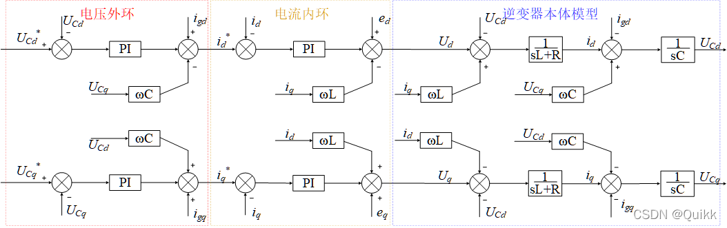
Usage （8） The following block diagram can be drawn .

   According to the inverter body model, double PI Control schematic diagram , Because by Combine after decoupling PI controller Precise control can be achieved .

Grid connected inverter PI Controller constant value tracking

about PI controller
$$\begin{gathered} G_{(s)}=K_P(1+\frac{K_i}{s})=\frac{K_{P}s+K_P{K}_i}{s} \\ G(j\omega )=\frac{K_{P}j\omega +K_P{K}_i}{j\omega } \end{gathered}$$
therefore ：
$$G(j0)=\frac{K_{P}j0+K_P{K}_i}{j0}=\infty$$
At this time, the closed-loop transmittal is ：
$$A=\frac{G_{(j0)}}{1+G_{(j0)}}=1$$
therefore PI The controller pair frequency is 0 The signal of （ DC signal ） Can achieve Tracking without static error ！ Therefore, in the above process, the inverter control model needs to be transformed to dq Axis , because dq Transformation is based on PLL The output voltage angle is transformed , So the three-phase current is dq In coordinate system （d The shaft component is the current amplitude ,q The axis component is zero ）. Decoupling is to eliminate other shaft pairs PI The impact of control .

Simulation results

SPWM Modulation signal ：

Output line voltage （ Before filter ）：

Load side phase voltage （0.1s Grid connection ,0.8s Given power step ）：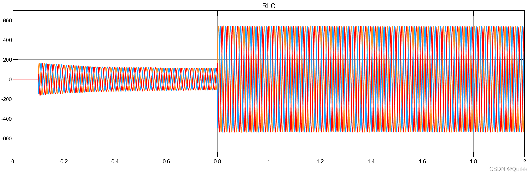

Output power ：

simulation model ： Model links