当前位置:网站首页>PI control of grid connected inverter (grid connected mode)
PI control of grid connected inverter (grid connected mode)
2022-07-02 09:37:00 【Quikk】
Grid connected inverter PI control
1. Inverter topology and mathematical model
The following figure shows the basic structure model of the inverter .
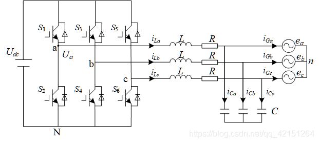
According to the model, write the mathematical model of the inverter as follows :
{ U a − L d i a d t − i a R − e a = 0 U b − L d i b d t − i b R − e b = 0 U c − L d i c d t − i c R − e c = 0 \begin{cases}{} U_a-L\frac{di_a}{dt}-i_aR-e_a=0\\ U_b-L\frac{di_b}{dt}-i_bR-e_b=0\\ U_c-L\frac{di_c}{dt}-i_cR-e_c=0 \end{cases} ⎩⎪⎨⎪⎧Ua−Ldtdia−iaR−ea=0Ub−Ldtdib−ibR−eb=0Uc−Ldtdic−icR−ec=0
2. Common transformations
2.1 abc- α β \alpha\beta αβ Transformation and its inverse transformation
The specific principle is not deduced here , Please refer to other materials .
[ U α U β ] = m × [ 1 − 1 2 − 1 2 0 3 2 − 3 2 ] [ U a U b U c ] \left[ \begin {matrix} U_\alpha\\ U_\beta \end{matrix}\right] =m \times \left[ \begin {matrix} 1 & -\frac{1}{2} & -\frac{1}{2}\\ 0 & \frac{\sqrt{3}}{2} & -\frac{\sqrt{3}}{2} \end{matrix} \right] \left[ \begin {matrix} U_a\\ U_b\\ U_c \end{matrix} \right] [UαUβ]=m×[10−2123−21−23]⎣⎡UaUbUc⎦⎤
m The value of is related to the system requirements ;
{ m = 2 3 work rate phase etc. change in m = 2 3 picture value phase etc. change in \begin {cases}{} m =\sqrt{\frac{2}{3}} & Equal power conversion \\ m =\frac{2}{3} & Equal amplitude transformation \end{cases} { m=32m=32 work rate phase etc. change in picture value phase etc. change in
In control , We often choose amplitude invariant algorithm for control .
When m = 2 3 m=\frac{2}{3} m=32 Correspondingly, there is inverse transformation :
[ U a U b U c ] = m × [ 1 0 − 1 2 3 2 − 1 2 − 3 2 ] [ U α U β ] \left[ \begin {matrix} U_a\\ U_b\\ U_c \end{matrix}\right]= m\times \left[ \begin {matrix} 1 & 0 \\ -\frac{1}{2} & \frac{\sqrt{3}}{2} \\ -\frac{1}{2} & -\frac{\sqrt{3}}{2} \end{matrix} \right] \left[ \begin {matrix} U_\alpha\\ U_\beta\\ \end{matrix} \right] ⎣⎡UaUbUc⎦⎤=m×⎣⎢⎡1−21−21023−23⎦⎥⎤[UαUβ]
2.2 α β \alpha\beta αβ-dq Axis transformation
[ U d U q ] = [ c o s φ s i n φ − s i n φ c o s φ ] [ U α U β ] \left[ \begin {matrix} U_d\\ U_q\\ \end{matrix} \right]= \left[ \begin {matrix} cos\varphi & sin\varphi \\ -sin\varphi & cos\varphi \end{matrix} \right] \left[ \begin {matrix} U_\alpha\\ U_\beta\\ \end{matrix} \right] [UdUq]=[cosφ−sinφsinφcosφ][UαUβ]
The corresponding inverse transformation is
[ U α U β ] = [ c o s φ − s i n φ s i n φ c o s φ ] [ U d U q ] \left[ \begin {matrix} U_\alpha\\ U_\beta\\ \end{matrix} \right]= \left[ \begin {matrix} cos\varphi & -sin\varphi \\ sin\varphi & cos\varphi \end{matrix} \right] \left[ \begin {matrix} U_d\\ U_q\\ \end{matrix} \right] [UαUβ]=[cosφsinφ−sinφcosφ][UdUq]
Here we need to pay attention to :
1. In a general way , In the control of the inverter, the grid voltage is oriented to d Axis , Therefore, the angle in the transformation formula is the phase angle of the power grid .
2. according to dq And α β \alpha\beta αβ The equal positions of the coordinate axes are different , There are different forms of transformation , Specific reference to . Like European electric four dq Transformation
2.3 abc-dq Transformation
[ U d U q ] = 2 3 [ c o s φ c o s ( φ − 2 3 π ) c o s ( φ + 2 3 π ) − s i n φ − s i n ( φ − 2 3 π ) − s i n ( φ + 2 3 π ) ] [ U a U b U c ] \left[ \begin {matrix} U_d\\ U_q\\ \end{matrix} \right] =\frac{2}{3} \left[ \begin {matrix} cos\varphi & cos(\varphi-\frac{2}{3}\pi) & cos(\varphi+\frac{2}{3}\pi) \\ -sin\varphi & -sin(\varphi-\frac{2}{3}\pi) & -sin(\varphi+\frac{2}{3}\pi) \end{matrix} \right] \left[ \begin {matrix} U_a\\ U_b\\ U_c \end{matrix} \right] [UdUq]=32[cosφ−sinφcos(φ−32π)−sin(φ−32π)cos(φ+32π)−sin(φ+32π)]⎣⎡UaUbUc⎦⎤
3.dq Equation of parallel inverter in coordinate system
Will type (1) Conduct dq Change can get :
[ U d U q ] = L d d t [ i a i b i c ] × T a b c _ d q + [ i d i q ] R + [ e d e q ] \left[ \begin {matrix} U_d\\ U_q\\ \end{matrix} \right] =L\frac{d}{dt} \left[ \begin {matrix} i_a \\ i_b\\ i_c \end{matrix} \right]\times T_{abc\_dq} + \left[ \begin {matrix} i_d\\ i_q\\ \end{matrix} \right]R + \left[ \begin {matrix} e_d\\ e_q\\ \end{matrix} \right] [UdUq]=Ldtd⎣⎡iaibic⎦⎤×Tabc_dq+[idiq]R+[edeq]
among :
d [ i a i b i c ] × T a b c _ d q d t = d [ i a i b i c ] d t × T a b c _ d q + d T a b c _ d q d t × [ i a i b i c ] \frac{d\left[ \begin {matrix} i_a \\ i_b\\ i_c\end{matrix}\right]\times T_{abc\_dq}}{dt}= \frac{d\left[ \begin {matrix} i_a \\ i_b\\ i_c \end{matrix} \right]}{dt}\times T_{abc\_dq} + \frac{dT_{abc\_dq}}{dt}\times \left[ \begin {matrix} i_a \\ i_b\\ i_c \end{matrix} \right] dtd⎣⎡iaibic⎦⎤×Tabc_dq=dtd⎣⎡iaibic⎦⎤×Tabc_dq+dtdTabc_dq×⎣⎡iaibic⎦⎤
among φ = ω t \varphi=\omega t φ=ωt
d T a b c _ d q d t = ω [ − s i n φ − s i n ( φ − 2 3 π ) − s i n ( φ + 2 3 π ) − c o s φ − c o s ( φ − 2 3 π ) − c o s ( φ + 2 3 π ) ] \frac{dT_{abc\_dq}}{dt}=\omega \left[ \begin {matrix} -sin\varphi & -sin(\varphi-\frac{2}{3}\pi) & -sin(\varphi+\frac{2}{3}\pi) \\ -cos\varphi & -cos(\varphi-\frac{2}{3}\pi) & -cos(\varphi+\frac{2}{3}\pi) \end{matrix} \right] dtdTabc_dq=ω[−sinφ−cosφ−sin(φ−32π)−cos(φ−32π)−sin(φ+32π)−cos(φ+32π)]
therefore :
d T a b c _ d q d t × [ i a i b i c ] = ω × [ i q − i d ] \frac{dT_{abc\_dq}}{dt}\times \left[ \begin {matrix} i_a \\ i_b\\ i_c \end{matrix} \right]= \omega \times \left[ \begin {matrix} i_q \\ -i_d\\ \end{matrix} \right] dtdTabc_dq×⎣⎡iaibic⎦⎤=ω×[iq−id]
Substitute into the original formula to get :
d [ i a i b i c ] d t × T a b c _ d q = d [ i d i q ] d t − ω × [ i q − i d ] \frac{d\left[ \begin {matrix} i_a \\ i_b\\ i_c \end{matrix} \right]}{dt}\times T_{abc\_dq}= \frac{d\left[ \begin {matrix} i_d \\ i_q \\ \end{matrix} \right]}{dt}-\omega \times \left[ \begin {matrix} i_q \\ -i_d\\ \end{matrix} \right] dtd⎣⎡iaibic⎦⎤×Tabc_dq=dtd[idiq]−ω×[iq−id]
Then the mathematical model of the grid connected inverter is :
[ U d U q ] = L d d t [ i d i q ] − ω L × [ i q − i d ] + [ i d i q ] R + [ e d e q ] \left[ \begin {matrix} U_d\\ U_q\\ \end{matrix} \right] =L\frac{d}{dt}\left[ \begin {matrix} i_d \\ i_q\\ \end{matrix} \right] -\omega L \times \left[ \begin {matrix} i_q \\ -i_d\\ \end{matrix} \right] + \left[ \begin {matrix} i_d\\ i_q\\ \end{matrix} \right]R + \left[ \begin {matrix} e_d\\ e_q\\ \end{matrix} \right] [UdUq]=Ldtd[idiq]−ωL×[iq−id]+[idiq]R+[edeq]
namely :
{ U d = L d i d d t − ω L i q + R i d + e d U q = L d i q d t + ω L i d + R i q + e q \left\{ \begin{matrix} U_d = L\frac{di_d}{dt}-\omega Li_q+Ri_d+e_d\\ U_q = L\frac{di_q}{dt}+\omega Li_d+Ri_q+e_q \end{matrix} \right. { Ud=Ldtdid−ωLiq+Rid+edUq=Ldtdiq+ωLid+Riq+eq
Laplace transform can get :
{ U d = ( L s + R ) i d − ω L i q + e d U q = ( L s + R ) i q + ω L i d + e q \left\{ \begin{matrix} U_d = (Ls+R)i_d-\omega Li_q+e_d\\ U_q = (Ls+R)i_q+\omega Li_d+e_q \end{matrix} \right. { Ud=(Ls+R)id−ωLiq+edUq=(Ls+R)iq+ωLid+eq
4. Closed loop control
According to the inverter model , The input to be built is Id* Output is Ud Of PI Control link . Decoupling control of inverter can be realized .( First modification : Decoupling is actually introduced here to eliminate the influence of disturbance on the system , such as Grid voltage 、 Current feedforward wait , After elimination, the system will become simple to pass PI Link to correct the system .)
introduce PI Links are available :
{ U d = ( K p + K i s ) ( i d ∗ − i d ) − ω L i q + e d U q = ( K p + K i s ) ( i q ∗ − i q ) + ω L i d + e q \left\{ \begin{matrix} U_d = (Kp+\frac{Ki}{s})(i_d^*-i_d)-\omega Li_q+e_d\\ U_q = (Kp+\frac{Ki}{s})(i_q^*-i_q)+\omega Li_d+e_q \end{matrix} \right. { Ud=(Kp+sKi)(id∗−id)−ωLiq+edUq=(Kp+sKi)(iq∗−iq)+ωLid+eq
The following figure shows the overall control block diagram of the inverter system :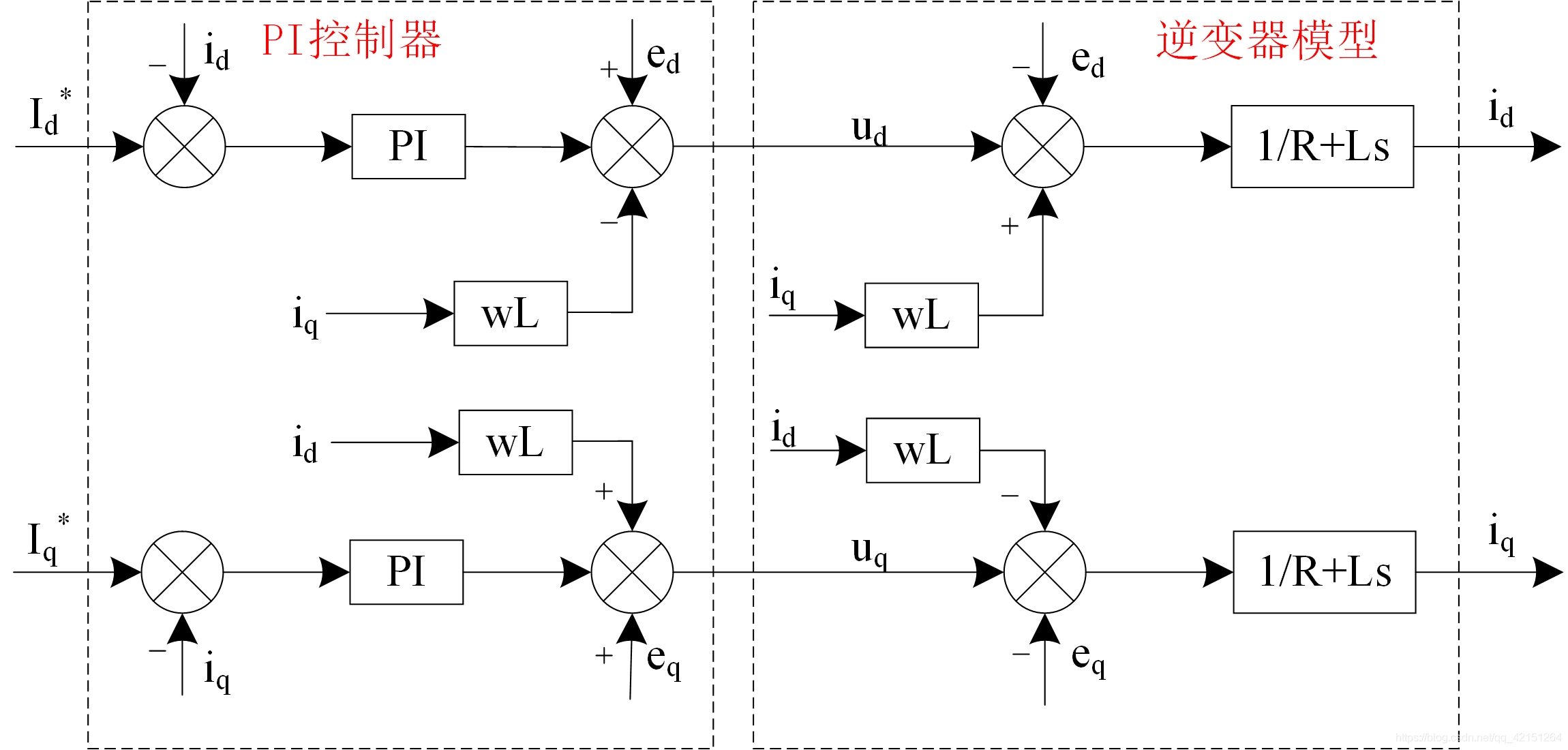
According to this equation, we can build PI Current closed-loop control block diagram :

Some current models are bidirectional rectifier models in current control , That is, the current is defined as the flow of the power grid to the DC side . At this time, the circuit equation will change , The control block diagram will also happen . At this time, the control model is :
{ U d = − ( K p + K i s ) ( i d ∗ − i d ) + ω L i q + e d U q = − ( K p + K i s ) ( i q ∗ − i q ) − ω L i d + e q \left\{ \begin{matrix} U_d = -(Kp+\frac{Ki}{s})(i_d^*-i_d)+\omega Li_q+e_d\\ U_q = -(Kp+\frac{Ki}{s})(i_q^*-i_q)-\omega Li_d+e_q \end{matrix} \right. { Ud=−(Kp+sKi)(id∗−id)+ωLiq+edUq=−(Kp+sKi)(iq∗−iq)−ωLid+eq
Build the corresponding circuit according to the model .
5. Simulated main circuit
According to the relevant parameters , Build the simulation main circuit :

Simulation results :
Current amplitude given waveform :

Output current waveform :
Output power waveform

Model links
Model links , I need to take it myself : Grid connected inverter PI control
边栏推荐
猜你喜欢

Number structure (C language -- code with comments) -- Chapter 2, linear table (updated version)
图像识别-数据清洗
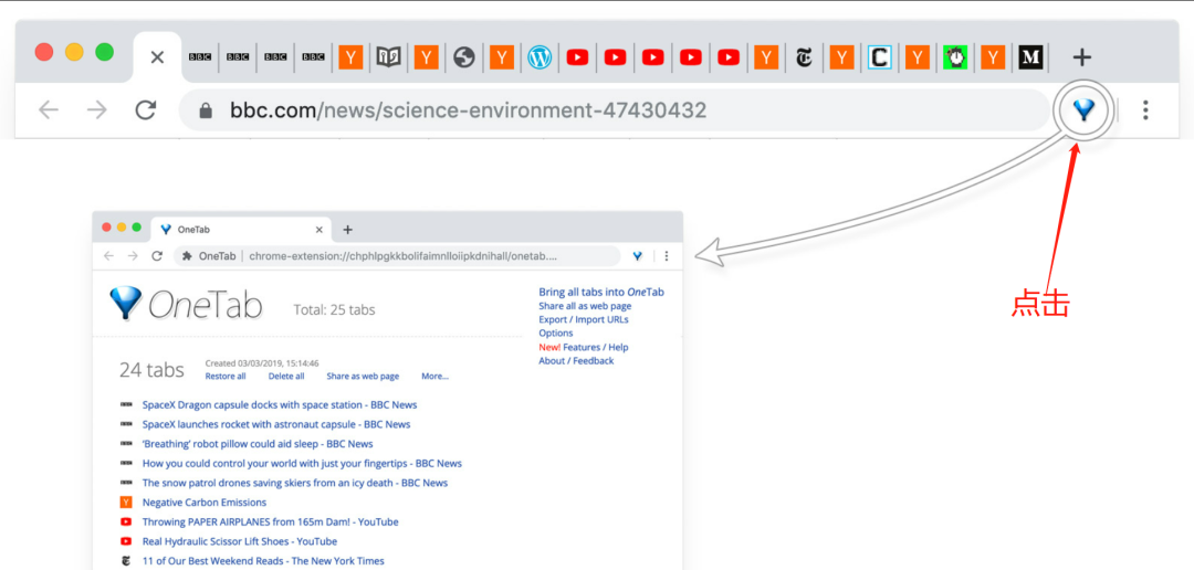
Chrome browser tag management plug-in – onetab

三相逆变器离网控制——PR控制
![[go practical basis] gin efficient artifact, how to bind parameters to structures](/img/c4/44b3bda826bd20757cc5afcc5d26a9.png)
[go practical basis] gin efficient artifact, how to bind parameters to structures

Chrome browser plug-in fatkun installation and introduction

MySQL事务

Microservice practice | teach you to develop load balancing components hand in hand

Solution to amq4036 error in remote connection to IBM MQ

Idea view bytecode configuration
随机推荐
What are the waiting methods of selenium
kinect dk 获取CV::Mat格式的彩色RGB图像(openpose中使用)
Mathematics in machine learning -- point estimation (I): basic knowledge
每天睡前30分钟阅读Day5_Map中全部Key值,全部Value值获取方式
自定義Redis連接池
Required request body is missing: (cross domain problem)
保存视频 opencv::VideoWriter
YOLO物体识别,生成数据用到的工具
Demand delineation executive summary
JDBC review
记录一下初次使用Xray的有趣过程
Failed to configure a DataSource: ‘url‘ attribute is not specified and no embedd
Machine learning practice: is Mermaid a love movie or an action movie? KNN announces the answer
Oracle modify database character set
微服务实战|声明式服务调用OpenFeign实践
Learn combinelatest through a practical example
Microservice practice | load balancing component and source code analysis
三相逆变器离网控制——PR控制
Oracle delete tablespace and user
道阻且长,行则将至