当前位置:网站首页>Hands on deep learning (40) -- short and long term memory network (LSTM)
Hands on deep learning (40) -- short and long term memory network (LSTM)
2022-07-04 09:41:00 【Stay a little star】
List of articles
One 、 Long and short term memory network (LSTM)
The earliest method used to deal with the problems of long-term information preservation and short-term input jump in implicit variable models (long short-term memory LSTM). It has the same properties as many gated cycle units .LSTM Than GRU More complicated , But its ratio GRU Early birth 20 About years ago .
1.1 Gated memory unit
LSTM Introduced storage unit (memory cell), Abbreviated as unit (cell). Some literatures think that storage unit is a special type of hidden state , They have the same shape as the hidden state , It is designed to record additional information . In order to control the storage unit , We need many doors . One of the doors is used to read entries from the unit . Let's call this Output gate (output gate). Another gate is used to decide when to read data into the unit . Let's call this Input gate (input gate). Last , We need a mechanism to reset the contents of the unit , from Oblivion gate (forget gate) To manage . The motivation for this design is the same as that of the gated cycle unit , That is, it can decide when to remember or ignore the input in the hidden state through a special mechanism . Let's see how this works in practice .
- Oblivion gate : Turn the value toward 0 The direction decreases
- Input gate : Decide whether to ignore input data
- Output gate : Decide whether to use hidden state
1.2 Input gate 、 Forgetting gate and output gate
Just like in the gated cycle unit , The input of the current time step and the hidden state of the previous time step are sent into the long-term and short-term memory network gate as data , As shown in the figure below . They consist of three with sigmoid Activate the full connection layer processing of the function , To calculate the input gate 、 Forget the values of gate and output gate . therefore , The values of these three doors are ( 0 , 1 ) (0, 1) (0,1) Within the scope of .

mathematical description , Suppose there is h h h Hidden units , Batch size is n n n, The number of inputs is d d d. therefore , Input is X t ∈ R n × d \mathbf{X}_t \in \mathbb{R}^{n \times d} Xt∈Rn×d, The hidden state of the previous time step is H t − 1 ∈ R n × h \mathbf{H}_{t-1} \in \mathbb{R}^{n \times h} Ht−1∈Rn×h. Accordingly , Time step t t t The door of is defined as follows : The input gate is I t ∈ R n × h \mathbf{I}_t \in \mathbb{R}^{n \times h} It∈Rn×h, The forgetting door is F t ∈ R n × h \mathbf{F}_t \in \mathbb{R}^{n \times h} Ft∈Rn×h, The output gate is O t ∈ R n × h \mathbf{O}_t \in \mathbb{R}^{n \times h} Ot∈Rn×h. Their calculation method is as follows :
I t = σ ( X t W x i + H t − 1 W h i + b i ) , F t = σ ( X t W x f + H t − 1 W h f + b f ) , O t = σ ( X t W x o + H t − 1 W h o + b o ) , \begin{aligned} \mathbf{I}_t &= \sigma(\mathbf{X}_t \mathbf{W}_{xi} + \mathbf{H}_{t-1} \mathbf{W}_{hi} + \mathbf{b}_i),\\ \mathbf{F}_t &= \sigma(\mathbf{X}_t \mathbf{W}_{xf} + \mathbf{H}_{t-1} \mathbf{W}_{hf} + \mathbf{b}_f),\\ \mathbf{O}_t &= \sigma(\mathbf{X}_t \mathbf{W}_{xo} + \mathbf{H}_{t-1} \mathbf{W}_{ho} + \mathbf{b}_o), \end{aligned} ItFtOt=σ(XtWxi+Ht−1Whi+bi),=σ(XtWxf+Ht−1Whf+bf),=σ(XtWxo+Ht−1Who+bo),
among W x i , W x f , W x o ∈ R d × h \mathbf{W}_{xi}, \mathbf{W}_{xf}, \mathbf{W}_{xo} \in \mathbb{R}^{d \times h} Wxi,Wxf,Wxo∈Rd×h and W h i , W h f , W h o ∈ R h × h \mathbf{W}_{hi}, \mathbf{W}_{hf}, \mathbf{W}_{ho} \in \mathbb{R}^{h \times h} Whi,Whf,Who∈Rh×h It's a weight parameter , b i , b f , b o ∈ R 1 × h \mathbf{b}_i, \mathbf{b}_f, \mathbf{b}_o \in \mathbb{R}^{1 \times h} bi,bf,bo∈R1×h Is the offset parameter .
1.3 Candidate memory unit
Next , Design memory unit . Since the operation of various doors has not been specified , So let's start with Candidate memory unit (candidate memory cell) C ~ t ∈ R n × h \tilde{\mathbf{C}}_t \in \mathbb{R}^{n \times h} C~t∈Rn×h. Its calculation is similar to that of the three doors described above , But use tanh \tanh tanh Function as activation function , The value range of the function is ( − 1 , 1 ) (-1, 1) (−1,1). The following export is in the time step t t t Equation at :
C ~ t = tanh ( X t W x c + H t − 1 W h c + b c ) , \tilde{\mathbf{C}}_t = \text{tanh}(\mathbf{X}_t \mathbf{W}_{xc} + \mathbf{H}_{t-1} \mathbf{W}_{hc} + \mathbf{b}_c), C~t=tanh(XtWxc+Ht−1Whc+bc),
among W x c ∈ R d × h \mathbf{W}_{xc} \in \mathbb{R}^{d \times h} Wxc∈Rd×h and W h c ∈ R h × h \mathbf{W}_{hc} \in \mathbb{R}^{h \times h} Whc∈Rh×h It's a weight parameter , b c ∈ R 1 × h \mathbf{b}_c \in \mathbb{R}^{1 \times h} bc∈R1×h Is the offset parameter .
The diagram of candidate memory units is as follows

1.4 Memory unit
In the gating cycle unit , There is a mechanism to control input and forgetting ( Or skip ). Similarly , In short-term and long-term memory networks , There are also two doors for this purpose : Input gate I t \mathbf{I}_t It Control how much is used from C ~ t \tilde{\mathbf{C}}_t C~t New data for , And forget the door F t \mathbf{F}_t Ft Control how many old memory units are retained C t − 1 ∈ R n × h \mathbf{C}_{t-1} \in \mathbb{R}^{n \times h} Ct−1∈Rn×h The content of . Use the same technique of multiplying by elements as before , The following updated formula is obtained :
C t = F t ⊙ C t − 1 + I t ⊙ C ~ t . \mathbf{C}_t = \mathbf{F}_t \odot \mathbf{C}_{t-1} + \mathbf{I}_t \odot \tilde{\mathbf{C}}_t. Ct=Ft⊙Ct−1+It⊙C~t.
If the forgetting door is always 1 1 1 And the input gate is always 0 0 0, Then the memory unit of the past C t − 1 \mathbf{C}_{t-1} Ct−1 Will be saved over time and passed to the current time step . This design is introduced to alleviate the gradient disappearance problem , And better capture the long-distance dependence in the sequence .
So we get the flow chart , as follows .

1.5 Hidden state
Last , We need to define how to calculate hidden states H t ∈ R n × h \mathbf{H}_t \in \mathbb{R}^{n \times h} Ht∈Rn×h. This is where the output gate works . In short-term and long-term memory networks , It's just a memory unit tanh \tanh tanh Gated version of . This ensures that H t \mathbf{H}_t Ht The value of is always in the interval ( − 1 , 1 ) (-1, 1) (−1,1) Inside .
H t = O t ⊙ tanh ( C t ) . \mathbf{H}_t = \mathbf{O}_t \odot \tanh(\mathbf{C}_t). Ht=Ot⊙tanh(Ct).
As long as the output gate is close to 1 1 1, We can effectively transfer all memory information to the prediction part , For the output gate, close to 0 0 0, We only keep all the information in the storage unit , And there is no further process to perform .
The following is a graphical demonstration of all data streams .

Two 、 From zero LSTM
import torch
from torch import nn
from d2l import torch as d2l
# load data iter
batch_size, num_steps = 32, 35
train_iter, vocab = d2l.load_data_time_machine(batch_size, num_steps)
2.1 Initialize model parameters
#  Casually initialize , The standard deviation used here is 0.01 Initialization of Gaussian distribution , Offset use 0
def get_lstm_params(vocab_size,num_hiddens,device):
    num_inputs = num_outputs = vocab_size

    def normal(shape):
        return torch.randn(size=shape,device=device)*0.01
    def three():
        return(normal((num_inputs,num_hiddens)),
               normal((num_hiddens,num_hiddens)),
               torch.zeros(num_hiddens,device=device))
    W_xi, W_hi, b_i = three()  #  Enter the door parameters
    W_xf, W_hf, b_f = three()  #  Forget the door parameters
    W_xo, W_ho, b_o = three()  #  Output gate parameters
    W_xc, W_hc, b_c = three()  #  Candidate memory cell parameters
    #  Output layer parameters
    W_hq = normal((num_hiddens, num_outputs))
    b_q = torch.zeros(num_outputs, device=device)
    #  Additional gradient
    params = [
        W_xi, W_hi, b_i, W_xf, W_hf, b_f, W_xo, W_ho, b_o, W_xc, W_hc, b_c,
        W_hq, b_q]
    for param in params:
        param.requires_grad_(True)
    return params
2.2 Define the network model
In the initialization function ,LSTM The hidden state of needs to return an additional memory unit , The value of its cell is 0, Shape is ( Batch size , Number of hidden units ).
def init_lstm_state(batch_size,num_hiddens,device):
    return (torch.zeros((batch_size,num_hiddens),device=device),
            torch.zeros((batch_size,num_hiddens),device=device))
#  The definition of the actual model is the same as the previous definition , Provide three doors and an additional memory unit . Only hidden states are passed to the output layer , The memory unit is not directly involved in the output calculation
def lstm(inputs,state,params):
    [W_xi, W_hi, b_i, W_xf, W_hf, b_f, W_xo, W_ho, b_o, W_xc, W_hc, b_c,W_hq, b_q] = params
    (H,C) = state
    outputs = []
    for X in inputs:
        I = torch.sigmoid(([email protected]_xi)+([email protected]_hi)+b_i)
        F = torch.sigmoid((X @ W_xf) + (H @ W_hf) + b_f)
        O = torch.sigmoid((X @ W_xo) + (H @ W_ho) + b_o)
        C_tilda = torch.tanh((X @ W_xc) + (H @ W_hc) + b_c)
        C = F * C + I * C_tilda
        H = O * torch.tanh(C)
        Y = (H @ W_hq) + b_q
        outputs.append(Y)
    return torch.cat(outputs, dim=0), (H, C)
2.3 Training and forecasting
vocab_size, num_hiddens, device = len(vocab), 256, d2l.try_gpu()
num_epochs, lr = 500, 1
model = d2l.RNNModelScratch(len(vocab), num_hiddens, device, get_lstm_params,init_lstm_state, lstm)
d2l.train_ch8(model, train_iter, vocab, lr, num_epochs, device)
perplexity 1.1, 49112.9 tokens/sec on cuda:0
time traveller for so it will be convenient to speak of himwas e
traveller abcerthen thing the time traveller held in his ha

2.4 Concise implementation
num_inputs = vocab_size
lstm_layer = nn.LSTM(num_inputs, num_hiddens)
model = d2l.RNNModel(lstm_layer, len(vocab))
model = model.to(device)
d2l.train_ch8(model, train_iter, vocab, lr, num_epochs, device)
perplexity 1.1, 281347.3 tokens/sec on cuda:0
time traveller for so it will be convenient to speak of himwas e
travelleryou can show black is white by argument said filby

The long-term and short-term memory network is a typical implicit variable autoregressive model with important state control . Many variants have been proposed over the years , for example , Multi-storey 、 Residual connection 、 Different types of regularization . However , Due to the long-distance dependence of the sequence , Train short-term and long-term memory networks and other sequence models ( Cycle control unit, e.g ) The cost of is quite high . In the following content , We will encounter alternative models that can be used in some cases , Such as Transformer.
Summary
- There are three types of gates in long-term and short-term memory networks : Input gate 、 Forgetting gate and output gate controlling information flow .
- The hidden layer outputs of long-term and short-term memory networks include “ Hidden state ” and “ Memory unit ”. Only the hidden state is passed to the output layer , The memory unit is completely internal information .
- Long-term and short-term memory networks can alleviate gradient disappearance and gradient explosion .
practice
- How do you need to change the model to generate the appropriate words , Not a sequence of characters
At the time of input , We need to treat words as vocab Encoding , But in that case ,onehot The size of the code may need to become very large . Data processing , Give each word a corresponding number , Number this onehot Coding can also .
- Given the hidden layer dimension , Compare the gating cycle unit 、 The computational cost of long-term and short-term memory networks and conventional Recurrent Neural Networks . Pay special attention to the cost of training and reasoning .
- Since candidate memory units are used tanh \tanh tanh Function to ensure that the hedging range is ( − 1 , 1 ) (-1,1) (−1,1) Between , So why do hidden states need to be used again tanh \tanh tanh Function to ensure that the output value range is ( − 1 , 1 ) (-1,1) (−1,1) Between ?
I t = σ ( X t W x i + H t − 1 W h i + b i ) , F t = σ ( X t W x f + H t − 1 W h f + b f ) , O t = σ ( X t W x o + H t − 1 W h o + b o ) , \begin{aligned} \mathbf{I}_t &= \sigma(\mathbf{X}_t \mathbf{W}_{xi} + \mathbf{H}_{t-1} \mathbf{W}_{hi} + \mathbf{b}_i),\\ \mathbf{F}_t &= \sigma(\mathbf{X}_t \mathbf{W}_{xf} + \mathbf{H}_{t-1} \mathbf{W}_{hf} + \mathbf{b}_f),\\ \mathbf{O}_t &= \sigma(\mathbf{X}_t \mathbf{W}_{xo} + \mathbf{H}_{t-1} \mathbf{W}_{ho} + \mathbf{b}_o), \end{aligned} ItFtOt=σ(XtWxi+Ht−1Whi+bi),=σ(XtWxf+Ht−1Whf+bf),=σ(XtWxo+Ht−1Who+bo), C ~ t = tanh ( X t W x c + H t − 1 W h c + b c ) , \tilde{\mathbf{C}}_t = \text{tanh}(\mathbf{X}_t \mathbf{W}_{xc} + \mathbf{H}_{t-1} \mathbf{W}_{hc} + \mathbf{b}_c), C~t=tanh(XtWxc+Ht−1Whc+bc), C t = F t ⊙ C t − 1 + I t ⊙ C ~ t . \mathbf{C}_t = \mathbf{F}_t \odot \mathbf{C}_{t-1} + \mathbf{I}_t \odot \tilde{\mathbf{C}}_t. Ct=Ft⊙Ct−1+It⊙C~t. H t = O t ⊙ tanh ( C t ) . \mathbf{H}_t = \mathbf{O}_t \odot \tanh(\mathbf{C}_t). Ht=Ot⊙tanh(Ct).
边栏推荐
- How can people not love the amazing design of XXL job
- C # use gdi+ to add text with center rotation (arbitrary angle)
- Regular expression (I)
- Pueue data migration from '0.4.0' to '0.5.0' versions
- Explanation of for loop in golang
- Function comparison between cs5261 and ag9310 demoboard test board | cost advantage of cs5261 replacing ange ag9310
- Log cannot be recorded after log4net is deployed to the server
- Leetcode (Sword finger offer) - 35 Replication of complex linked list
- Modules golang
- Tkinter Huarong Road 4x4 tutorial II
猜你喜欢
ASP. Net to access directory files outside the project website
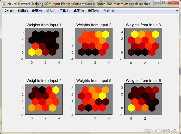
Matlab tips (25) competitive neural network and SOM neural network
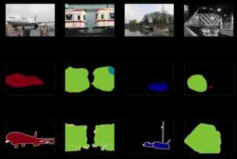
Hands on deep learning (32) -- fully connected convolutional neural network FCN

2022-2028 global gasket metal plate heat exchanger industry research and trend analysis report
2022-2028 global probiotics industry research and trend analysis report
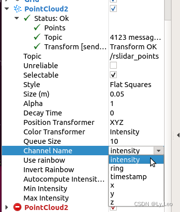
pcl::fromROSMsg报警告Failed to find match for field ‘intensity‘.
Kubernetes CNI 插件之Fabric
2022-2028 global visual quality analyzer industry research and trend analysis report
2022-2028 global edible probiotic raw material industry research and trend analysis report
2022-2028 global small batch batch batch furnace industry research and trend analysis report
随机推荐
Write a jison parser from scratch (2/10): learn the correct posture of the parser generator parser generator
Are there any principal guaranteed financial products in 2022?
Hands on deep learning (35) -- text preprocessing (NLP)
Global and Chinese market of air fryer 2022-2028: Research Report on technology, participants, trends, market size and share
JDBC and MySQL database
Summary of the most comprehensive CTF web question ideas (updating)
智慧路灯杆水库区安全监测应用
Explanation of closures in golang
Four common methods of copying object attributes (summarize the highest efficiency)
C # use gdi+ to add text to the picture and make the text adaptive to the rectangular area
Golang Modules
Hands on deep learning (34) -- sequence model
Pueue data migration from '0.4.0' to '0.5.0' versions
C # use smtpclient The sendasync method fails to send mail, and always returns canceled
Fatal error in golang: concurrent map writes
品牌连锁店5G/4G无线组网方案
`Example of mask ` tool use
Reading notes on how to connect the network - hubs, routers and routers (III)
2022-2028 global gasket plate heat exchanger industry research and trend analysis report
After unplugging the network cable, does the original TCP connection still exist?