当前位置:网站首页>Matlab 信号处理【问答随笔·2】
Matlab 信号处理【问答随笔·2】
2022-07-07 21:50:00 【鹅毛在路上了】
1. Matlab 简单插值、拟合方法
答:
clc,clear,close all;
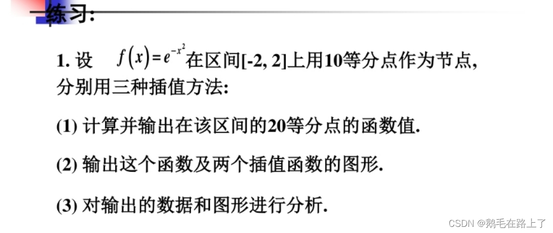
x = linspace(-2,2,10);
y = exp(-x.^2);
figure(1)
stem(x,y,"LineWidth",1.5)
grid on
title('f(x)')
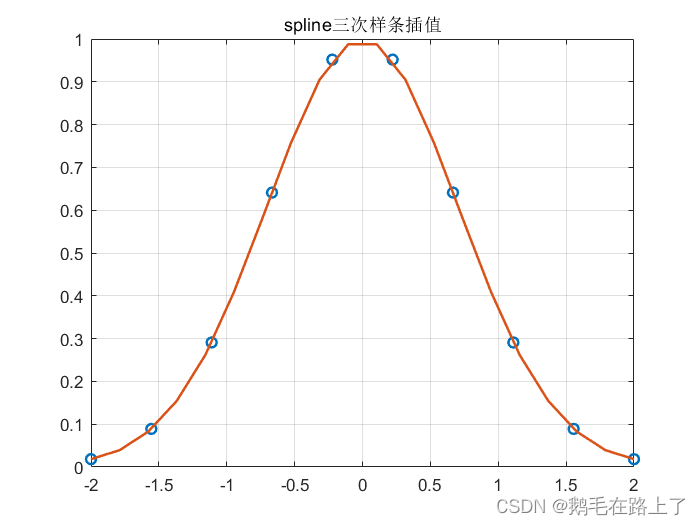
%interp1线性插值
xq = linspace(-2,2,20);
vq1 = interp1(x,y,xq);
figure(2)
plot(x,y,'o',xq,vq1,':.',"LineWidth",1.5);
xlim([-2 2]);
grid on
title('interp1线性插值');
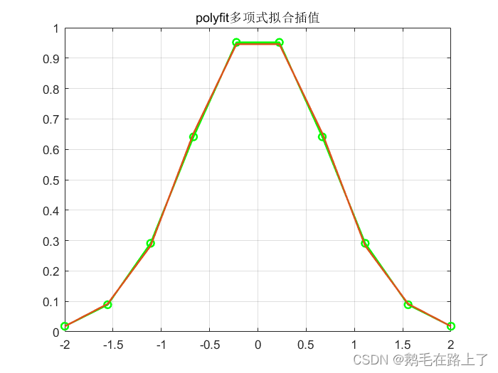
%polyfit多项式拟合插值
p = polyfit(x,y,7);
y1 = polyval(p,x);
figure(3)
plot(x,y,'g-o',"LineWidth",1.5)
hold on
plot(x,y1,"LineWidth",1.5)
hold off
xlim([-2 2]);
grid on
title('polyfit多项式拟合插值');
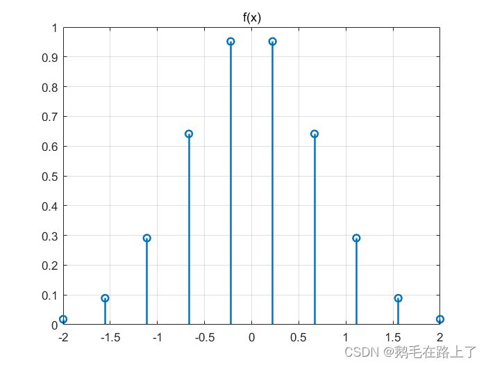
%spline三次样条插值
yy = spline(x,y,xq);
figure(4)
plot(x,y,'o',xq,yy,"LineWidth",1.5)
xlim([-2 2]);
grid on
title('spline三次样条插值');
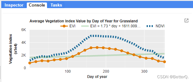
2. 数字信号处理实验——FIR滤波器设计
问:已知输入信号为混有噪声的信号
x(t)=sin(250πt)+cos(500πt)+cos(700πt)
①画出输入信号时域波形和频谱图,并指出其包含的频率成分(以Hz为单位);
②假定输入信号的中间频率成分为噪声信号,请问应如何设计数字滤波器处理该混合信号,给出合理的设计指标并说明理由,画出滤波器的频响特性:要求两种以上的实现方案。
③用(2)中设计的滤波器完成滤波并验证设计方案,画出滤波器输出信号时域波形和频谱图。
答:
clc,clear,close all;
t = -0.08:0.0001:0.08;
n = -100:100;
L = length(n);
fs = 1000;
x0 = sin(2*pi*125.*n/fs);  %时域采样后的信号t=nT=n/fs
x1 = cos(2*pi*250.*n/fs);
x2 = cos(2*pi*350.*n/fs);
x3 = x0 + x1 + x2;
%时域信号
figure(1)
subplot(411)
plot(t,sin(2*pi*125.*t),"LineWidth",1.5)
grid on
subplot(412)
plot(t,cos(2*pi*250.*t),"LineWidth",1.5)
grid on
subplot(413)
plot(t,cos(2*pi*350.*t),"LineWidth",1.5)
grid on
subplot(414)
plot(t,sin(2*pi*125.*t)+cos(2*pi*250.*t)+cos(2*pi*350.*t),"LineWidth",1.5)
grid on
%滤波器设计
wn = 3/5;  %截止频率wn为3/5pi(300Hz),wn = 2pi*f/fs
N = 60;  %阶数选择
hn = fir1(N-1,wn,boxcar(N));  %10阶FIR低通滤波器
figure(2)
freqz(hn,1);
figure(3)
y = fftfilt(hn,x3);  %经过FIR滤波器后得到的信号
plot(n,y,"LineWidth",1.5)
grid on
%频谱分析
X = fft(x3); %未滤波前的频谱
p2 = abs(X/L);
p1 = p2(1:L/2+1);
p1(2:end-1) = 2*p1(2:end-1);
Y = fft(y);  %输出信号的fft
P2 = abs(Y/L);
P1 = P2(1:L/2+1);
P1(2:end-1) = 2*P1(2:end-1);
f = fs*(0:(L/2))/L;
figure(4)
subplot(211)
plot(f,p1,"LineWidth",1.5)
title('Single-Sided Amplitude Spectrum of X(t)')
xlabel('f (Hz)')
ylabel('|p1(f)|')
grid on
subplot(212)
plot(f,P1,"LineWidth",1.5)
title('Single-Sided Amplitude Spectrum of Y(t)')
xlabel('f (Hz)')
ylabel('|P1(f)|')
grid on
时域波形:分别为125(2pi*125=250pi)、250和350Hz的余弦信号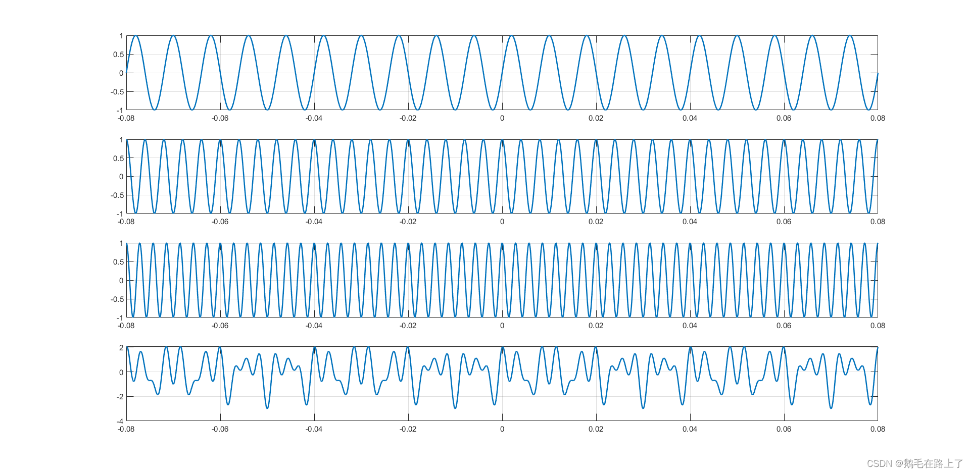
截止频率为300Hz的FIR低通滤波器: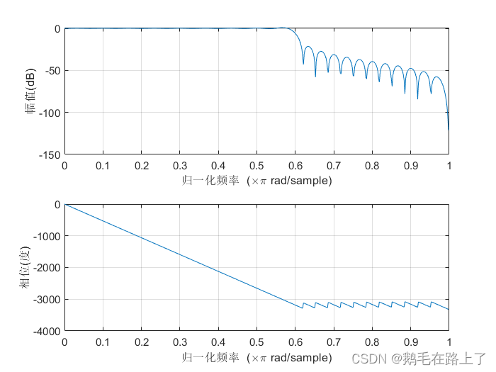
滤波前和滤波后的频谱: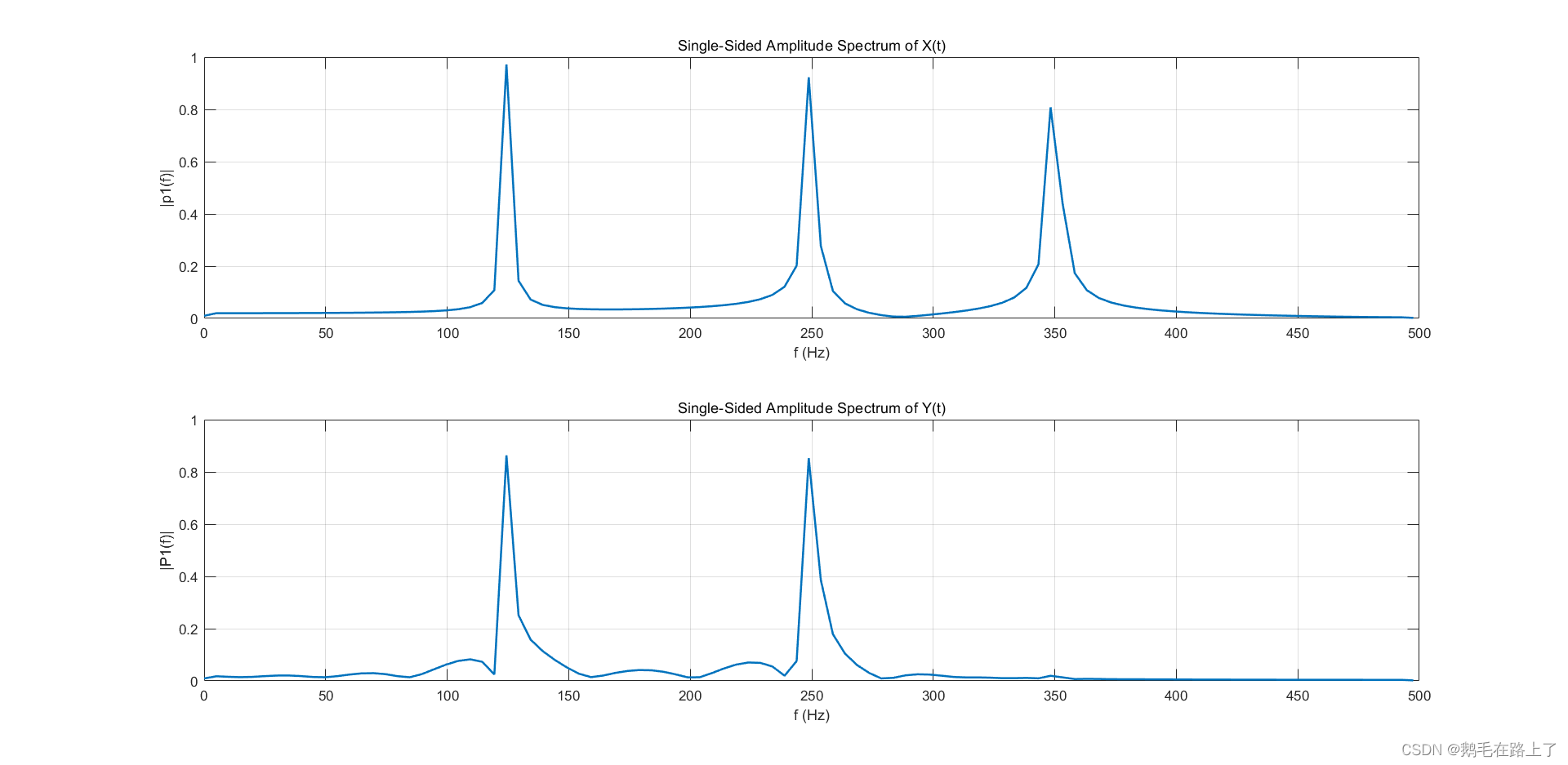
滤波后的时域信号: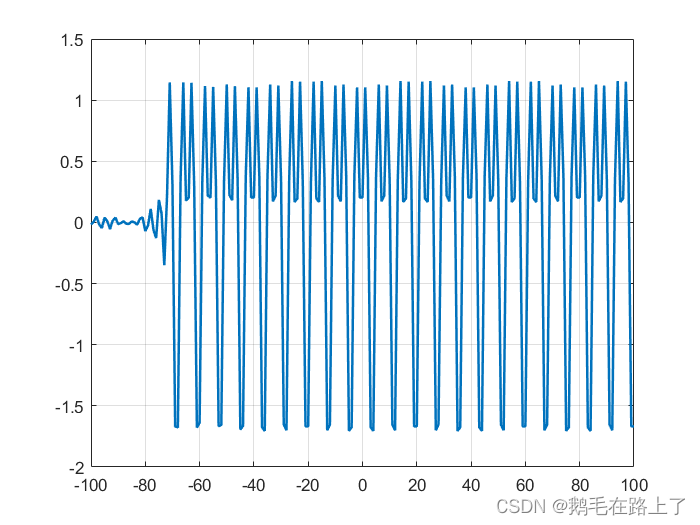
3. Matlab做的热力图为什么不是顺滑的过渡?——伪彩图函数pcolor()的用法
问题相关代码:
clear; clc; close all
[,,raw ] = xlsread('体育设施热力图数据.xlsx');
mat = cell2mat(raw(2:end, 2:end));
imagesc(mat); %生成热图
c=colorbar;
colormap hot;
ylabel(c,'Population Heat');
caxis([1 11]) %更改右侧颜色条最大最小值
xticks(1:13) %x轴分成13等分
xticklabels(raw(1,2:end))
yticks(1:15)
yticklabels(raw(2:end,1))
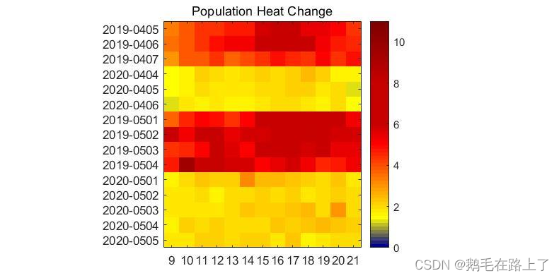
预期效果: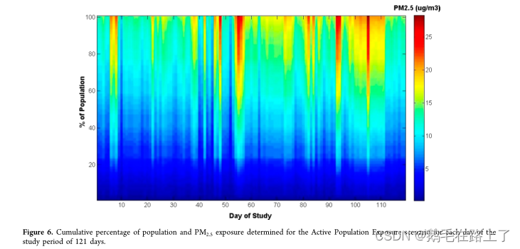
答:可能是数据量较少的原因,预期效果不仅仅是用的imagesc(),更像是颜色插值后的伪彩图,建议尝试pcolor():
clc,clear,close all;
data=round(rand(1,900)*100);
data=reshape(data,10,90);
h=pcolor(data);
h.FaceColor = 'interp';
set(h,'LineStyle','none');
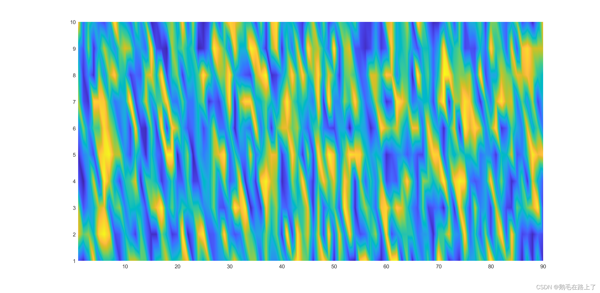
clc,clear,close all;
data=round(rand(1,900)*100);
data=reshape(data,10,90);
h=pcolor(data);
h.FaceColor = 'interp';
colormap jet;
colorbar;
set(h,'LineStyle','none');
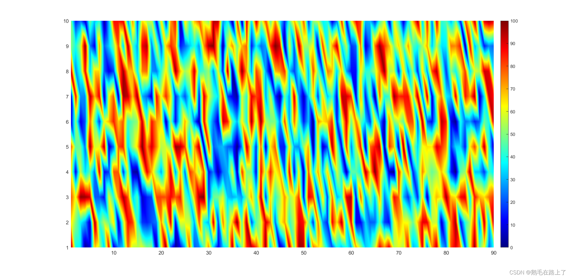
伪彩图函数pcolor()的用法:pcolor官方文档
边栏推荐
猜你喜欢
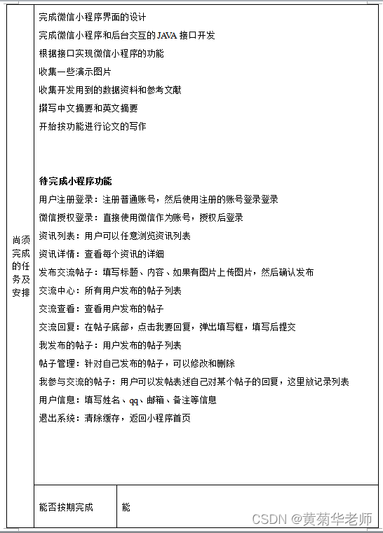
Wechat forum exchange applet system graduation design completion (7) Interim inspection report
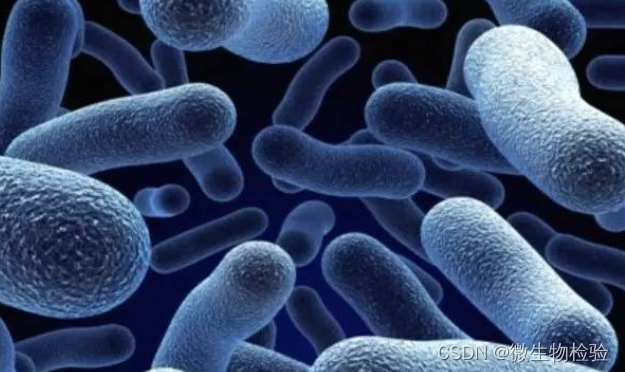
肠道里的微生物和皮肤上的一样吗?

Online interview, how to better express yourself? In this way, the passing rate will be increased by 50%~
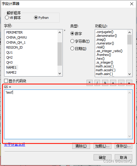
ArcGIS: field assignment_ The attribute table field calculator assigns values to fields based on conditions
![Cause analysis and solution of too laggy page of [test interview questions]](/img/33/2c2256fd98b908ddaf5573f644ad7f.png)
Cause analysis and solution of too laggy page of [test interview questions]

Digital collections accelerated out of the circle, and marsnft helped diversify the culture and tourism economy!

Personal statement of testers from Shuangfei large factory: is education important for testers?
Are the microorganisms in the intestines the same as those on the skin?
GEE(四):计算两个变量(影像)之间的相关性并绘制散点图
PMP project management exam pass Formula-1
随机推荐
网络安全-beef
Cascade-LSTM: A Tree-Structured Neural Classifier for Detecting Misinformation Cascades-KDD2020
二叉树(Binary Tree)
网格(Grid)
Wechat forum exchange applet system graduation design (2) applet function
网络安全-钓鱼
USB(十五)2022-04-14
网络安全-burpsuit
聊聊支付流程的设计与实现逻辑
网络安全-对操作系统进行信息查询
Brush question 4
Cases of agile innovation and transformation of consumer goods enterprises
网络安全-永恒之蓝
PMP project management exam pass Formula-1
One question per day - pat grade B 1002 questions
Network security sqlmap and DVWA explosion
Introduction to redis and jedis and redis things
kubernetes的简单化数据存储StorageClass(建立和删除以及初步使用)
十四、数据库的导出和导入的两种方法
数据库每日一题---第22天:最后一次登录