当前位置:网站首页>Matlab learning notes
Matlab learning notes
2022-07-07 00:27:00 【Evergreen AAS】
notes :
- Although the documentation is comprehensive , But this article is mainly to speed up in one day , So please forgive me for my shortcomings .
- The code is based on vscode/py 3.6 Called matlab terminal
Basic mathematical operations and matrix operations
Basic grammar
Variable
- No declaration required
- use = Assign a value to a variable
Variable name
- Variable names are case sensitive ( I don't know if it's because windows Why
- Variable names can only be used by [
0~9,a~z,A~z,_] form , And the variable name cannot start with a number . - Reserved variables are not suitable for variable names
- Use
iskeywordCommand can view program keywords , These keywords are not allowed to be used as variable names .
- Use
Variable | significance |
|---|---|
ans | The result of the last sentence |
i,j | Complex operator ,( We need to pay attention here ) |
Inf | infinite |
eps | Floating point relative precision , namely 1.0 The distance to the next floating-point number ( The value is 2.2204e-16) |
NaN | The digital |
pi | PI |
Variable names should not override built-in function names
stay MATLAB in , Call priority of variables (calling priority) Higher than function , Therefore, variable names should not override built-in functions .
for example :
cos = 'changqingaas';
cos(8)
% disp(['ans is ', num2str(ans)])
clear; %  If a function is overwritten by a variable name , Call clear < Variable name > You can unbind the variable name on the function name
cos(8)
% disp(['ans is ', num2str(ans)])
notes :clear It's a dangerous order , Because if you do not add parameters after this command , It means to clear all variables in the current workspace .
 Output :

ans =

    'n'


ans =

   -0.1455
Variable type
logical,char,numeric,cell,struct And the array or matrix composed of them .
Display format of numeric variables
Numeric variables , Default to double Stored in form .
Can pass format < Display format > Change the display format of numeric variables .
MATLAB Command line
- Use end of line
;Suppress output :- Use after a line of command
;Suppress output , Otherwise, the calculation result will be displayed on the terminal .
- Use after a line of command
- | command | effect | Running results | | ———- | —————————————————————————————— | —————————————————————————————— | |
clc| Clear the output of the terminal | | |clear| By default, all variables in the current workspace are cleared | | |who| Display all variables in the workspace in a simplified format | Your variable is : ans | |whos| Display all variables in the workspace in a complex format | Name Size Bytes Class Attributes ans 1x1 8 double | | which | Check the location of the built-in function source code file , AndeditCommand can be combined to view the source code of built-in functions . | |
Use MATLAB Do numerical calculations
Use MATLAB Calculate mathematical expressions
- After the mathematical expression is calculated , Its value is stored in the variable ans
- log Express ln
- exp(x) Express e^x
MATLAB Built in mathematical functions
- MATLAB Built in arithmetic operation function
- Basic operation :
- Add :
+,sum,cumsum,movsum - reduce :
-,diff - ride :
.*,*,prod,cumprod - except :
./,.\,/,\ - chengfang :
.^,^
- Add :
- Modulus operation :
mod,rem,idivide,ceil,fix,floor,round
- Basic operation :
- MATLAB Built in trigonometric function
- sine : sin,sind,sinpi,asin,asind,sinh,asinh
- cosine : cos,cosd,cospi,acos,acosd,cosh,acosh
- tangent : tan,tand,atan,atand,atan2,atan2d,tanh,atanh
- Cosecant : csc,cscd,acsc,acscd,csch,acsch
- Secant : sec,secd,asec,asecd,sech,asech
- Cotangent : cot,cotd,acot,acotd,coth,acoth
- hypotenuse : hypot
- transformation : deg2rad,rad2deg,cart2pol,cart2sph,pol2cart,sph2cart
- MATLAB Built in exponential logarithmic function :
- exp,expm1,log,log10,log1p,log2,nextpow2,nthroot,pow2,reallog,realpow,realsqrt,sqr
- MATLAB Built in complex function :
- abs,angle,complex,conj,cplxpair,i,imag,isreal,j,real,sign,unwrap
Use MATLAB Do matrix operations
Define the matrix
Input the matrix to the terminal
stay MATLAB in , Use [] Enclose the matrix contents to be input , Use spaces or commas , Separate inline variables , Use ; Separate each line .
Use the colon operator to create a vector
Use the colon operator : You can create a long vector , The syntax is as follows :
for example :
Define a special matrix
command | The result |
|---|---|
eye(n) | Get one n × n The identity matrix of |
zeros(n1, n2) | Get one n1 × n2 Of all the 0 matrix |
ones(n1, n2) | Get one n1 × n2 Of all the 1 matrix |
diag(vector) | Get a vector vector The content in is the diagonal matrix of diagonal |
The index of the matrix
- MATLAB The matrix in is represented by Column Sequentially stored . And the index subscript is from 1 Start .
- Matrices can be indexed in two ways : Index by one dimension and index by two dimensions . For a general matrix , The index order is as follows : \begin{bmatrix} 1 or (1,1) & 4 or (1,2) & 7 or (1,3) \\ 2 or (2,1) & 5 or (2,2) & 8 or (2,3) \\ 3 or (3,1) & 6 or (3,2) &9 or (3,3) \end{bmatrix}
- The index of matrix can use colon
:, Means to select all rows or columns . - The index of a matrix can be one or two vectors , Indicates that all rows or columns in the selected vector . | Primitive matrix | Indexes | The result || —————————————————————————————— | ———————- | ———————————————————————————- || \begin{bmatrix} 1 & 2 & 3 \\ 4 & 5 & 6\\ 7 & 8 & 9 \end{bmatrix}\begin{bmatrix} 1 & 2 & 3 \\ 4 & 5 & 6\\ 7 & 8 & 9 \end{bmatrix}\begin{bmatrix} 1 & 2 & 3 \\ 4 & 5 & 6\\ 7 & 8 & 9 \end{bmatrix}\begin{bmatrix} 1 & 4 \\ 7 & 2\end{bmatrix}\begin{bmatrix} 1 & 2 & 3 \\ 4 & 5 & 6\\ 7 & 8 & 9 \end{bmatrix}\begin{bmatrix} 1 & 2 & 3 \\ 4 & 5 & 6\\ 7 & 8 & 9 \end{bmatrix}\begin{bmatrix} 1 & 2 & 3 \\ 4 & 5 & 6 \end{bmatrix}\begin{bmatrix} 1 & 2 & 3 \\ 4 & 5 & 6\\ 7 & 8 & 9 \end{bmatrix}\begin{bmatrix} 1 & 2 \\ 7 & 8 \end{bmatrix}
Matrix operations
Operator of operation matrix
Operator | operation | form | Example |
|---|---|---|---|
+ | Add matrix and vector | A+b | [6 3] + 2 = [8 5] |
- | Matrix subtracts from vector | A-b | [6 3] - 2 = [4 1] |
+ | Add the matrix to its corresponding position | A+B | [6 3] + [4 8] = [10 11] |
- | The matrix is subtracted from the corresponding position of the matrix | A-B | [6 3] - [4 8] = [2 -5] |
* | Matrix Matrix Multiplication | A*B | [6 3] * [4 8]' = 48 |
.* | Multiply the matrix by its corresponding position | A.*B | [6 3] * [4 8] = [24 24] |
/ | Matrix and matrix right division ( Equivalent to A*inv(B)) | A/B | [6 3] / [4 8] = 0.6 |
\ | Matrix and matrix left division ( Equivalent to inv(A)*B) | A\B | [6 3] / [4 8] = [0.06667 1.3333; 0 0] |
./ | The matrix and the corresponding position of the matrix are divided by | A./B | [6 3] ./ [4 8] = [1.5 0.375] |
.\ | The matrix and the corresponding position of the matrix are divided by left | A.\B | [6 3] .\ [4 8] = [0.6667 2.6667] |
^ | Matrix and vector power | A^b | [1 2; 3 4]^3 = [37 54; 81 118] |
.^ | Matrix and matrix corresponding position power | A.^B | [1 2; 3 4].^[1 2; 3 4] = [1 4; 27 256] |
Function of operation matrix
For the following matrix
A=\begin{bmatrix} 1 & 2 & 3 \\ 0 & 5 & 6 \\ 7 & 0 & 9 \end{bmatrix}
Operate to demonstrate common functions of the operation matrix
For the above functions , Except for the first parameter , Other parameters are optional .
Structured programming and function definition
Structured programming
Process control statements and logical operators
Flow control statement | effect |
|---|---|
if, elseif, else | if if The statement is true , Execute clause |
switch, case, otherwise | according to switch The content of the statement determines which clause to execute |
while | Repeat the clause until while The condition in is false |
for | Execute the clause a fixed number of times |
try, catch | Execute clauses and catch exceptions during execution |
break | Out of the loop |
continue | Go directly to the next cycle |
end | End clause |
pause | Suspend program |
return | Return to the calling function |
All the above loops and conditional statements should end with end closed .
MATLAB There are also the following logical operators :
Operator | significance | ||
|---|---|---|---|
== | be equal to | ||
~= | It's not equal to | ||
&& | And ( Support logic short circuit ) | ||
` | ` | or ( Support logic short circuit ) |
Example of process control statement
if sentence :
if condition1
	statement1
elseif condition2
	statement2
else
	statement3
end
switch sentence
switch expression
    case value1
        statement1
    case value2
        statement2
    otherwise
        statement
end
while sentence
while expression
	statement
end
for sentence
for variable = start:increment:end
	commands
end
break sentence
x = 2; k = 0; error = inf;
error_threshold = 1e-32;

while error > error_threshold

    if k > 100
        break
    end

    x = x - sin(x) / cos(x);
    error = abs(x - pi);
    k = k + 1;
end
Try to pre allocate memory space when using circular statements
Problems that should be paid attention to when writing scripts
Add a statement at the beginning of the script to empty the workspace
At the beginning of each script , The following statement should be added , Clear the workspace cache and traces of previous program runs :
clear all	%  Clear variables in the workspace memory
close all 	%  Close the image drawn by the program before
clc			%  Clear the output of the program on the terminal before
Semicolons should be added after operations and assignment statements ; Suppress output
Semicolons should be added to all operations and assignment statements ; Suppress output , If you need to output a variable to the terminal , It should be called disp Method .
Use ellipsis ... Splice multiple lines
stay MATLAB in , Ellipsis ... You can splice multiple lines of statements into one line , Using this statement flexibly can improve the readability of the code .
function
Similar to scripts , Functions can be stored Function name .m In file , It can also be defined in memory in the form of a function handle .
See built-in functions
We can use which Command to view the location of the built-in function source code file , And edit Command can be combined to view the source code of built-in functions .
Run the following statement to open MATLAB Built in mean Function source file :
edit(which('mean.m')) With Function name .m File form definition function
stay MATLAB The format of the function defined in the file is as follows :
function [ Output variable name ] =  Function name ( Enter variable name )
%  Documentation for functions

 function code
functionIt's a keyword , Declare that what is saved in this file is a function .The input variableandOutput variablesnonessential , Functions can have no input variables , You can also have no output variables .Function nameShould and.mSame file name , And does not contain special characters ( It's better not to have Chinese ).
MATLAB Built in function parameters
Function parameter | significance |
|---|---|
imputname | Enter a list of variable names |
mfilename | Function source code file name |
nargin | Enter the number of variables |
nargout | Number of output variables |
varargin | Variable length input parameter list |
varargout | Variable length output parameter list |
MATLAB It does not provide the syntax of specifying default parameter values and function overloading in other high-level languages , But use the built-in function parameters mentioned above flexibly , You can specify the default parameter value and method overloading to a certain extent :
MATLAB Function definition example 1
The surface program is used to calculate the displacement of a free falling body :x = x_{0} + v_{0}t + \frac{1}{2} g t^2
function x = freebody(x0,v0,t)
% calculation of free falling
% x0: initial displacement in m
% v0: initial velocity in m/sec
% t: the elapsed time in sec
% x: the depth of falling in m
x = x0 + v0.*t + 1/2*9.8*t.*t;
This function demonstrates a MATLAB Programming skills : Try to use .* Instead of *, Because the former is not only for parameters t Scalar case is available , Also for variables t In the case of vectors or matrices .
freebody(0, 0, 2)			%  obtain  19.6000
freebody(0, 0, [0 1 2 3])	%  obtain  [0 4.9000 19.6000 44.1000]
freebody(0, 0, [0 1; 2 3])	%  obtain  [0 4.9000; 19.6000 44.1000]
MATLAB Function definition example 2
The following function realizes the conversion from Fahrenheit temperature to Celsius temperature , This function can identify the number of input samples to be converted , When the number of samples to be converted is 0 when , Exit function .
function F2C()
while 1
    F_degree = input('tempreature in Fahrenheit: ', 's');
    F_degree = str2num(F_degree);
    if isempty(F_degree)
        return
    end
    C_degree = (F_degree-32)*5/9;
    disp(['tempreature in Celsius: ' num2str(C_degree)])
end
Define a function in the form of a function handle
We can also define functions in the form of function handles , This is closer to the mathematical definition of function , The syntax is as follows :
Function handle = @( The input variable ) Output variables
You can call this method directly through the function handle .
f = @(x) exp(-2*x);
x = 0:0.1:2;
plot(x, f(x));
Data type and file reading and writing
data type
MATLAB The main data types in are as follows :
value type (numeric)
MATLAB The supported value types are shown in the following table :
value type | describe |
|---|---|
double | Double precision floating point |
single | Single-precision floating-point |
int8 | 8 Bit signed integer |
int16 | 16 Bit signed integer |
int32 | 32 Bit signed integer |
int64 | 64 Bit signed integer |
uint8 | 8 Bit unsigned integer |
uint16 | 16 Bit unsigned integer |
uint32 | 32 Bit unsigned integer |
uint64 | 64 Bit unsigned integer |
stay MATLAB in , Variables of numeric type are defaulted to double Type of , You can use type conversion to convert it to other numeric types .
n = 3;
class(n)

n = int8(3);
class(n)
Output :
ans =
    'double'
ans =
    'int8'
String type (char)
stay MATLAB in , The string type consists of a pair of single quotation marks ' Wrap a paragraph of text to define . standard ASCII Characters can be converted to corresponding ASCII code .
s1 = 'h';
uint16(s1)	%  obtain  104
Strings are stored in memory in the form of a character matrix , You can index the matrix and assign values to it :
str1 = 'hello';
str2 = 'world';

str3 = [str1 str2];
size(str3)		%  obtain  [1 10]

str4 = [str1; str2];
size(str4)		%  obtain  [2 5]
str = 'aardvark';
'a' == str				%  obtain  [1 1 0 0 0 1 0 0]
str(str == 'a') = 'Z'	%  obtain  'ZZrdvZrk'
Structure (structure)
stay MATLAB in , The structure is a key value pair
The basic use of structures
- Similar to most programming languages ,MATLAB Use
.To access the fields in the structure :
student.name = 'John Doe';
student.id = '[email protected]';
student.number = 301073268;
student.grade = [100, 75, 73; ...
                 95, 91, 85.5; ...
                 100, 98, 72];
student
Using subscript expressions on the structure list can expand or reduce the structure list .
student.name = 'John Doe';
student.id = '[email protected]';
student.number = 301073268;
student.grade = [100, 75, 73; 95, 91, 85.5; 100, 98, 72];

student

student(2).name = 'Ann Lane';
student(2).id = '[email protected]';
student(2).number = 301078853;
student(2).grade = [95 100 90; 95 82 97; 100 85 100];

student(1) = [] %  Delete student The first item on the list
Structures can be cascaded , That is, the value of the field in the structure can also be the structure :
A = struct('data', [3 4 7; 8 0 1], ...
'nest', struct('testnum', 'Test 1', ...
'xdata', [4 2 8], ...
'ydata', [7 1 6]));
A(2).data = [9 3 2; 7 6 5];
A(2).nest.testnum = 'Test 2';
A(2).nest.xdata = [3 4 2];
A(2).nest.ydata = [5 0 9];

A
Common functions of structures
function | effect |
|---|---|
struct | Create structure |
struct2cell | Convert the structure to a cell array |
cell2struct | Convert the cell array into a structure |
isstruct | Determine whether a variable is a structure |
structfun | Apply a function to each field of the structure |
fieldnames | Get all field names of the structure |
isfield | Determine whether the structure contains a field |
getfield | Get the value of a field in the structure |
setfield | Assign a value to a field in the structure |
rmfield | Delete a field in the structure |
orderfields | Sort the structure fields |
Cell array (cell)
stay MATLAB in , A cell array is a data structure that can hold different types of elements , Be similar to Python Lists in languages .
Basic use of cellular arrays
Use {} Define a cell array like a matrix :
A = { [1 4 3; 0 5 8; 7 2 9]		'Anne Smith' ;...
3+7i		-pi:pi:pi}
A(1,1)={[1 4 3; 0 5 8; 7 2 9]};
A(1,2)={'Anne Smith'};
A(2,1)={3+7i};
A(2,2)={-pi:pi:pi};A{1,1}=[1 4 3; 0 5 8; 7 2 9];
A{1,2}='Anne Smith';
A{2,1}=3+7i;
A{2,2}=-pi:pi:pi;
AThe above three methods are equivalent , The second way is to use Cell index assignment , The third way is to use Content index assignment .
- There are two ways to access data in a cellular array , Namely : Cell index
()and Content index{}Because the subset of cell array is still cell array , In the use of indexer content , We need to point out that we are going to visit a Sub cell array still The contents in the corresponding area of the cell array .- Use Cell index
(), What we get is a Sub cell array .- Use Content index
{}, What we get is The contents in the corresponding area of the cell array .
- Use Content index
- Use Cell index
Common functions of cell array
Common functions of cell array
function | effect |
|---|---|
cell | Create a cell array |
iscell | Determine whether a variable is a cellular array |
cell2mat | Turn the cell array into a matrix |
cell2struct | Turn the cell array into a structure |
mat2cell | Converts an array to an array of cells of a specified size |
num2cell | Convert the array to a cell array of the same size |
struct2cell | Convert the structure to a cell array |
celldisp | Recursively display the contents of the cell array |
cellplot | Draw the structure of cell array in image form |
cellfun | Apply a function to each cell of the cell array |
among mat2cell Function can specify the size of each cell in the cell array when converting .
a = magic(3)

b = num2cell(a)
%  obtain
% [8] [1] [6]
% [3] [5] [7]
% [4] [9] [2]

c = mat2cell(a, [1 2], [2, 1])
%  obtain
% [1x2 double] [6]
% [2x2 double] [2x1 double]
High dimensional cell array
A three-dimensional cell array can have That's ok (row), Column (column), layer (layer) Three dimensions . When indexing a cell array , The order of priority from high to low is : That's ok → Column → layer .
Use cat Function can splice a cell array on a specified dimension .
A function that determines the data type of a variable
The following functions can judge the type of variables :
function | effect |
|---|---|
isinteger | Judge whether the input parameter is an integer array |
islogical | Judge whether the input parameter is a logical quantity array |
isnumeric | Judge whether the input parameter is a numeric array |
isreal | Judge whether the input parameter is a real array |
ischar | Judge whether the input parameter is a character array |
iscell | Judge whether the input parameter is a cell array |
isfloat | Determine whether the input array is a floating-point array |
ishandle | Determine whether the input array is a valid graphic handle |
isempty | Determine whether the input array is empty |
isprime | Determine which array elements are prime numbers |
isnan | Determine which array elements are NaN |
isinf | Determine which array elements are Inf |
isequal | Determine whether the array is equal |
File read and write
The supported file types are as follows :
The contents of the document | Extension | Function to read the file | Write function to file |
|---|---|---|---|
MATLAB data | *.mat | load | save |
Excel form | *.xls,*.xlsx | xlsread | xlswrite |
Space separated numbers | *.txt | load | save |
Reading and writing MATLAB Formatted data
MATLAB The data in the workspace can be in *.mat The format is saved in a file . Use save Function stores data in a file , Use load Function to read data from a file .
saveThe syntax of the function is as follows :save(filename,variables)Put the variablevariablesStored in a file in binary form .save(filename,variables,'-ascii')Put the variablevariablesSave in text form .
loadThe syntax of the function is as follows :load(filename)Read data from binary form file .load(filename,'-ascii')Read data from a text file .
The parameter filename and variables All in string format , If not specified variables Parameters , Then save all variables in the current workspace into a file .
Complex data formats , Such as
structandcell, Storage in binary format is not supported .
Reading and writing Excel form
Use xlsread and xlswrite Functions can be read and written Excel data , The grammar is as follows :
Read Excel The syntax of the document :[num,txt,raw] = xlsread(filename,sheet,xlRange)
Score = xlsread('04Score.xlsx')
Score = xlsread('04Score.xlsx', 'B2:D4')
[Score Header] = xlsread('04Score.xlsx')
write in Excel The grammar of :xlswrite(filename,A,sheet,xlRange)
M = mean(Score);
xlswrite('04Score.xlsx', M, 1, 'E2:E4');
xlswrite('04Score.xlsx', {'Mean'}, 1, 'E1');
Basic drawing
Drawing and decoration of drawing lines
Use plot() Function to draw lines
stay MATLAB in , Use plot() Function to draw lines , Its grammar is :
plot(x,y,LineSpec)
LineSpec: Line setting of drawing line , Three designations Linetype , The sign and Color Of Setter Make a string , The setting character does not distinguish the order . For details, please refer to Official documents .
Line symbols | Linetype setter | Mark | Tag setter | Color | Color setter |
|---|---|---|---|---|---|
- | Solid line ( Default ) | o | circle | y | yellow |
-- | Dotted line | plus | m | magenta | |
: | Dotted line | * | asterisk | c | Blue |
-. | Point line | . | spot | r | Red |
x | Cross | g | green | ||
s | square | b | Blue | ||
d | The diamond | w | white | ||
^ | Upper triangle | k | black | ||
v | Lower triangle | ||||
> | Right triangle | ||||
< | Left triangle | ||||
p | Pentagonal | ||||
h | hexagon |
notes :Python Medium matplotlib The way of drawing is almost the same as here
Decorative lines
Use legend() Function to add a legend to the picture
Use legend(label1, ..., labelN) Function can add a legend to the image .
x=0:0.5:4*pi;
y=sin(x); h=cos(x); w=1./(1+exp(-x)); g=(1/(2*pi*2)^0.5).*exp((-1.*(x-2*pi).^2)./(2*2^2));
plot(x,y,'bd-' ,x,h,'gp:',x,w,'ro-' ,x,g,'c^-');		%  Draw multiple lines
legend('sin(x)','cos(x)','Sigmoid','Gauss function');	%  Add legend
Use title() and *label() Add titles and labels to the pictures
x = 0:0.1:2*pi; y1 = sin(x); y2 = exp(-x);
plot(x, y1, '--*', x, y2, ':o');
xlabel('t = 0 to 2\pi');
ylabel('values of sin(t) and e^{-x}')
title('Function Plots of sin(t) and e^{-x}');
legend('sin(t)','e^{-x}');
Use text() and annotation() Add notes to the picture
x = linspace(0,3); y = x.^2.*sin(x); plot(x,y);
line([2,2],[0,2^2*sin(2)]);
str = '$$ \int_{0}^{2} x^2\sin(x) dx $$';
text(0.25,2.5,str,'Interpreter','latex');
annotation('arrow','X',[0.32,0.5],'Y',[0.6,0.4]);
Control the axis , Borders and grids
command | effect |
|---|---|
grid on/off | Set mesh visibility |
box on/off | Set border visibility |
axis on/off | Set axis visibility |
axis normal | Restore default behavior , Set the properties of frame aspect ratio mode and data aspect ratio mode to automatic |
axis square | Use coordinate axes of the same length , Adjust the increment between data units accordingly |
axis equal | Use the same data unit length along each axis |
axis tight | Set the coordinate axis range equal to the data range , Make the axis frame closely around the data |
The following example demonstrates axis Effect of command :
t = 0:0.1:2*pi; x = 3*cos(t); y = sin(t);
subplot(2, 2, 1); plot(x, y); axis normal
subplot(2, 2, 2); plot(x, y); axis square
subplot(2, 2, 3); plot(x, y); axis equal
subplot(2, 2, 4); plot(x, y); axis equal tight
Draw multiple lines
Draw multiple lines on an image
By default , Every time you execute plot() Function will clear the result of the last drawing , Multiple execution plot() Only the last drawing will be retained .
We can use hold on and hold off The command controls the refresh of the drawing area , Make multiple drawing results remain in the drawing area at the same time .
hold on		%  Bring up the brush , Start drawing a set of pictures
plot(cos(0:pi/20:2*pi));
plot(sin(0:pi/20:2*pi));
hold off	%  Put down the paintbrush , This group of pictures has been drawn
Draw multiple images in one window
subplot
Operation of graphic objects
stay MATLAB in , Graphics are stored in memory in the form of objects , You can operate on it by getting its graphic handle .
Get graph handle
A graph handle is essentially a floating point number , You can uniquely identify a graphic object . The following functions are used to get the graphic handle .
Function | Purpose |
|---|---|
gca() | Get the handle of the current coordinate axis |
gcf() | Get the handle of the current image |
allchild(handle_list) | Get the handle of all child objects of this object |
ancestor(h,type) | Get the latest type Ancestor nodes of type |
delete(h) | Delete an object |
findall(handle_list) | Get the descendants of this object |
All drawing functions also return handles to graphic objects .
Manipulate graphic attributes through graphic handles
Use get() and set() Function can access and modify the attributes of graphic objects . visit Official documents You can view the properties of all graphic objects .
set(H,Name,Value)v = get(h,propertyName)
The following two examples demonstrate the use of graphic handles to manipulate graphic objects :
Change axis properties :
%  The first picture
set(gca, 'FontSize', 25);

%  The second picture
set(gca, 'XTick', 0:pi/2:2*pi);
set(gca, 'XTickLabel', 0:90:360);

%  The third picture
set(gca, 'FontName', 'symbol');
set(gca, 'XTickLabel', {'0', 'p/2', 'p', '3p/2', '2p'});
Change Linetype
h = plot(x,y);
set(h, 'LineStyle','-.', ...
	'LineWidth', 7.0, ...
	'Color', 'g');
Save the drawing to a file
Use saveas(fig,filename) The command saves drawing objects to a file , among fig For graphics handle ,filname For the file name .
saveas(gcf, 'myfigure.png')
Draw advanced charts
Two dimensional charts
Broken line diagram
function | Graphic description |
|---|---|
loglog() | x Axis and y The axes take logarithmic coordinates |
semilogx() | x The axis takes logarithmic coordinates ,y The axis takes linear coordinates |
semilogy() | x The axis takes linear coordinates ,y The axis takes logarithmic coordinates |
plotyy() | With two sets y Linear coordinate system of coordinate axis |
ploar() | Polar system |
Logarithmic coordinate system drawing line
The following example demonstrates the logarithmic coordinate system line :
x = logspace(-1,1,100); y = x.^2;

subplot(2,2,1);
plot(x,y);
title('Plot');

subplot(2,2,2);
semilogx(x,y);
title('Semilogx');

subplot(2,2,3);
semilogy(x,y);
title('Semilogy');

subplot(2,2,4);
loglog(x, y);
title('Loglog');
Logarithmic coordinate system can be added grid , To distinguish between linear coordinate system and logarithmic coordinate system .
set(gca, 'XGrid','on');
double y Axis line
plotyy() The return value of is array [ax,hlines1,hlines2], among :
axIt's a vector , Save the handle of two coordinate system objects .hlines1andhlines2They are the handles of two graph lines .
x = 0:0.01:20;
y1 = 200*exp(-0.05*x).*sin(x);
y2 = 0.8*exp(-0.5*x).*sin(10*x);
[AX,H1,H2] = plotyy(x,y1,x,y2);
set(get(AX(1),'Ylabel'),'String','Left Y-axis')
set(get(AX(2),'Ylabel'),'String','Right Y-axis')
title('Labeling plotyy');
set(H1,'LineStyle','--'); set(H2,'LineStyle',':');
Statistical charts
function | Graphic description |
|---|---|
hist() | Histogram |
bar() | Two dimensional histogram |
pie() | The pie chart |
stairs() | Stairs |
stem() | Needle pattern |
Histogram
Histogram
Use bar() and bar3() Function to draw two-dimensional and three-dimensional histograms respectively
x = [1 2 5 4 8]; y = [x;1:5];
subplot(1,3,1); bar(x); title('A bargraph of vector x');
subplot(1,3,2); bar(y); title('A bargraph of vector y');
subplot(1,3,3); bar3(y); title('A 3D bargraph');
histIt is mainly used to view the frequency distribution of variables , andbarIt is mainly used to view the statistical results of discrete quantities .
Use barh() Function can draw a histogram of vertical arrangement
x = [1 2 5 4 8];
y = [x;1:5];
barh(y);
title('Horizontal');
towards bar() Pass in 'stack' Parameter allows the histogram to be drawn in the form of a stack .
x = [1 2 5 4 8];
y = [x;1:5];
bar(y,'stacked');
title('Stacked');
The pie chart
Use pie() and pie3() You can draw two-dimensional and three-dimensional pie charts . Pass a bool The vector indicates whether each sector is offset .
a = [10 5 20 30];
subplot(1,3,1); pie(a);
subplot(1,3,2); pie(a, [0,0,0,1]);
subplot(1,3,3); pie3(a, [0,0,0,1]);
Ladder diagram and needle diagram : Draw a sequence of discrete numbers
stairs() and stem() Function is used to draw ladder graph and needle graph respectively , Used to represent a sequence of discrete numbers .
x = linspace(0, 4*pi, 40); y = sin(x);
subplot(1,2,1); stairs(y);
subplot(1,2,2); stem(y);
Three dimensional chart
Convert a two-dimensional map to a three-dimensional map
stay MATLAB in , All drawings are three-dimensional , A two-dimensional picture is just a projection of a three-dimensional picture . Click... In the graphics window Rotate 3D Button , You can drag and drop the mouse to view the 3D view of the drawing .
Convert a three-dimensional drawing to a two-dimensional drawing
Use imagesc() Function can convert a three-dimensional view into a two-dimensional top view , The height is indicated by the color of the dot .
[x, y] = meshgrid(-3:.2:3,-3:.2:3); z = x.^2 + x.*y + y.^2;

subplot(1, 2, 1)
surf(x, y, z);

subplot(1, 2, 2)
imagesc(z);
Use colorbar The command can add the legend of the corresponding relationship between color and height on the generated two-dimensional map , Use colormap Command can change the color scheme . For details, please refer to Official documents
Three dimensional drawing
Preparation before drawing a three-dimensional map
- Use
meshgrid()Generate 2D mesh
meshgrid() Function expands the two input vectors by corresponding row expansion and column expansion to obtain two augmented matrices , The binary function can be applied to this matrix .
x = -2:1:2;
y = -2:1:2;
[X,Y] = meshgrid(x,y)
Z = X.^2 + Y.^2
Draw 3D lines
Use plot3() Function to draw a three-dimensional surface , Input should be three vectors .
x=0:0.1:3*pi; z1=sin(x); z2=sin(2.*x); z3=sin(3.*x);
y1=zeros(size(x)); y3=ones(size(x)); y2=y3./2;
plot3(x,y1,z1,'r',x,y2,z2,'b',x,y3,z3,'g'); grid on;
xlabel('x-axis'); ylabel('y-axis'); zlabel('z-axis');
Draw a 3D face
Use mesh() and surf() The command can draw 3D faces , The former does not fill the mesh while the latter .
x = -3.5:0.2:3.5; y = -3.5:0.2:3.5;
[X,Y] = meshgrid(x,y);
Z = X.*exp(-X.^2-Y.^2);
subplot(1,2,1); mesh(X,Y,Z);
subplot(1,2,2); surf(X,Y,Z);
Draw contour lines of 3D graphics
Use contour() and contourf() Function can draw contour lines of 3D graphics , The former does not fill the mesh while the latter .
towards contour() The function can change the details of the image by passing in parameters or manipulating the graphic handle :
x = -3.5:0.2:3.5; y = -3.5:0.2:3.5;
[X,Y] = meshgrid(x,y); Z = X.*exp(-X.^2-Y.^2);

subplot(1,3,1); contour(Z,[-.45:.05:.45]); axis square;
subplot(1,3,2); [C,h] = contour(Z); clabel(C,h); axis square;
subplot(1,3,3); contourf(Z); axis square;
Use meshc() and surfc() Function can draw its contour lines when drawing a three-dimensional figure .
x = -3.5:0.2:3.5; y = -3.5:0.2:3.5;
[X,Y] = meshgrid(x,y); Z = X.*exp(-X.^2-Y.^2);

subplot(1,2,1); meshc(X,Y,Z);
subplot(1,2,2); surfc(X,Y,Z);
Draw a three-dimensional volume
Use patch() Function can draw a three-dimensional body .
v = [0 0 0; 1 0 0 ; 1 1 0; 0 1 0; 0.25 0.25 1; 0.75 0.25 1; 0.75 0.75 1; 0.25 0.75 1];
f = [1 2 3 4; 5 6 7 8; 1 2 6 5; 2 3 7 6; 3 4 8 7; 4 1 5 8];

subplot(1,2,1);
patch('Vertices', v, 'Faces', f, 'FaceVertexCData', hsv(6), 'FaceColor', 'flat');
view(3); axis square tight; grid on;

subplot(1,2,2);
patch('Vertices', v, 'Faces', f, 'FaceVertexCData', hsv(8), 'FaceColor','interp');
view(3); axis square tight; grid on
Perspective and lighting of three-dimensional drawings
Adjust the perspective
Use view() Function can adjust the perspective ,view() Function accepts two floating-point arguments , Represent two azimuth angles respectively azimuth and elevation.
sphere(50); shading flat;
material shiny;
axis vis3d off;
view(-45,20);
Symbolic operations
Create symbolic variables
Create symbolic numbers
Use sym Function can create symbolic numbers . Using symbolic numbers can accurately save irrational numbers , There will be no error .
sym(1/3)	%  obtain  1/3
1/3			%  obtain  0.3333
Saving irrational numbers as symbolic numbers can avoid the error of converting them into floating-point numbers :
sin(sym(pi))	%  obtain  0
sin(pi)			%  obtain  1.2246e-16
Create symbolic variables
Use sym and syms You can create symbolic variables , The difference lies in :
sym Only one symbolic variable can be created at a time , and syms You can create multiple symbolic variables at a time .
syms a		% sym Command can only create one symbolic variable
syms b c d	% syms Command can create multiple symbolic variables
If the specified symbolic variable already exists ,sym It will not retain its original value , and syms Will clear its value .
syms x y
f = x+y;	%  Implicitly create symbolic variables f
sym f		%  Do not empty variables f Original value , namely f = x + y
syms x y
f = x+y;	%  Implicitly create symbolic variables f
syms f		%  Empty variables f Original value , namely f = f
Use sym You can create a symbolic variable matrix .
A = sym('a', [2 5])	%  Create a 2*5 Symbolic variable matrix of
whos
The output is as follows :
A =
[ a1_1, a1_2, a1_3, a1_4, a1_5]
[ a2_1, a2_2, a2_3, a2_4, a2_5]


  Name      Size            Bytes  Class    Attributes
  A         2x5               112  sym
A combination of sym and syms You can quickly create a series of variables with subscripts
clear all
syms(sym('a', [1 5]))
whos
The output is as follows :
Name      Size            Bytes  Class    Attributes
a1        1x1                 8  sym
a2        1x1                 8  sym
a3        1x1                 8  sym
a4        1x1                 8  sym
a5        1x1                 8  sym
Symbolic operations
Simplification and substitution of symbolic expressions
Simplification of symbolic expressions
Use simplify() Functions can simplify symbolic expressions .
syms x a b c

simplify(sin(x)^2 + cos(x)^2);		%  obtain  1
simplify(exp(c*log(sqrt(a+b))));	%  obtain  (a + b)^(c/2)
The standard of expression simplification is uncertain , The following three functions simplify the expression according to different standards :
expand() Functions can expand expressions
syms x

f = (x ^2- 1)*(x^4 + x^3 + x^2 + x + 1)*(x^4 - x^3 + x^2 - x + 1);
expand(f);		%  obtain  x^10 - 1
factor() Functions can be factorized
syms x

g = x^3 + 6*x^2 + 11*x + 6;
factor(g);		%  obtain  (x + 3)*(x + 2)*(x + 1)
horner() Functions can change polynomials into nested forms
syms x

h = x^5 + x^4 + x^3 + x^2 + x;
horner(h);		%  obtain  x*(x*(x*(x*(x + 1) + 1) + 1) + 1)
Substitution of symbolic expressions
Use sub(expr, old, new) The function can express a symbolic expression expr Medium old Replace with new.
syms x y

f = x^2*y + 5*x*sqrt(y);
subs(f, x, 3);	%  obtain  9*y + 15*y^(1/2)
Find the analytical solution of the equation
Use solve(eqn,var) and solve(eqns,vars) The analytical solution of the equation can be obtained .
Solve the univariate equation
Use == Define an equation , And call solve Function solving .( If not specified == The value to the right of the symbol , Then the default right side of the equation is 0.)
syms x

eqn = x^3 - 6*x^2 == 6 - 11*x;
solve(eqn);		%  obtain  [1 2 3]
Solve multivariable equations
For multivariable equations , We need to specify which variable to solve .
syms x y

eqn = [6*x^2 - 6*x^2*y + x*y^2 - x*y + y^3 - y^2 == 0];
solve(eqn, y);	%  obtain  [1, 2*x, -3*x]
Solve equations
towards solve() The function can be introduced into the equation system to solve the equation .
syms u v

eqns = [2*u + v == 0, u - v == 1];
S = solve(eqns,[u v]);
The solution of the equation can be indexed by the variable name , And the solution can be substituted into other expressions .
S.u;				%  obtain  1/3
S.v;				%  obtain  -2/3
subs(3*v + u, S);	%  obtain  -3/5
Symbolic calculus
Find the limit
Use limit(expr, var, a) Function can evaluate the symbolic expression expr In variables var Tend to be a The limit of time , Add parameter 'left' or 'right' You can specify the left limit or the right limit .
syms x;
expr = 1/x;

limit(expr,x,0);			%  obtain NaN
limit(expr,x,0,'left');		%  obtain -Inf
limit(expr,x,0,'right');	%  obtain Inf
differential
Use diff(expr, var, n) Function can evaluate the symbolic expression expr The variable var Of n First order differential .
syms a b c x;
expr = a*x^2 + b*x + c;

diff(expr, a);		%  obtain  x^2
diff(expr, b);		%  obtain  x
diff(expr, x);		%  obtain  b + 2*a*x
diff(expr, x, 2);	%  obtain  2*a
integral
Use int(expr, var) Function can evaluate the symbolic expression expr The variable var The indefinite integral of . Use int(expr, var, [a, b]) Function can specify upper and lower bounds to calculate definite integral ,a and b It can be a symbolic expression .
syms x a b
expr = -2*x/(1+x^2)^2;

int(expr, x);			%  obtain  1/(x^2 + 1)
int(expr, x, [1, 2]);	%  obtain  -0.3
int(expr, x, [1, Inf]);	%  obtain  -0.5
int(expr, x, [a, b]);	%  obtain  1/(b^2 + 1) - 1/(a^2 + 1)
For some functions ,MATLAB Its integral cannot be obtained , At this time MATLAB Will return an unresolved (unsolved) Integral form of .
syms x
int(sin(sinh(x)));	%  An integral without solution ,MATLAB return  int(sin(sinh(x)),
Sum of series
Use symsum(expr, k, [a b]) Calculation series expr The index of k from a To b The sum of .
syms k x

symsum(k^2, k)			%  obtain  k^3/3 - k^2/2 + k/6
symsum(k^2, k, [0 10])	%  obtain  385
symsum(x^k/factorial(k),k,1,Inf)	%  obtain  exp(x) - 1
Taylor expansion
Use taylor(expr,var,a) Calculation expression expr stay var=a The Taylor series at .
syms x

taylor(exp(x))	%  obtain  x^5/120 + x^4/24 + x^3/6 + x^2/2 + x + 1
taylor(sin(x))	%  obtain  x^5/120 - x^3/6 + x
taylor(cos(x))	%  obtain  x^4/24 - x^2/2 + 1
The plot
You can draw images of symbolic expressions , Common drawing functions are as follows :
function | effect |
|---|---|
fplot() | Draw a two-dimensional line image of a symbolic expression |
fplot3() | Draw a 3D line image of a symbolic expression |
ezpolar() | Draw the polar marking image of the symbolic expression |
fmesh() | Draw a mesh image |
fsurf() | Draw a colored face image |
fcontour() | Draw a contour image |
fimplicit() | Draw an image of implicit functional relationships |
The following example shows the drawing of two-dimensional and three-dimensional line images
subplot(1, 2, 1)
syms x
f = x^3 - 6*x^2 + 11*x - 6;
fplot(f, x)

subplot(1, 2, 2)
syms t
fplot3(t^2*sin(10*t), t^2*cos(10*t), t)
The following example demonstrates the rendering of three-dimensional surfaces
syms x y
fsurf(x^2 + y^2)
The following example demonstrates the drawing of implicit function relation image
syms x y
eqn = (x^2 + y^2)^4 == (x^2 - y^2)^2;
fimplicit(eqn, [-1 1])
Numerical calculation
Numerical operation of polynomials
Use MATLAB Represents a polynomial
Use vectors to represent polynomials
stay MATLAB in , Polynomials can be represented by vectors , The elements in the vector are the coefficients of polynomials ( Descending order ): The first is the coefficient of the highest order of the polynomial , The last digit is the constant term .
For example, polynomials : f(x) = x^3 - 2x - 5f(x)=x3−2x−5
You can use vectors p = [1 0 -2 -5] Express .
Polynomial evaluation :polyval()
Use polyval(p, x) You can calculate polynomials p stay x The value at each point .
a = [9,-5,3,7]; x = -2:0.01:5;
f = polyval(a,x);
plot(x,f);
Multiplication of polynomials :conv()
Use conv(p1, p2) Function can be applied to two vectors p1 and p2 Convolution multiplication , Used to calculate the multiplication of polynomials .
For example, polynomials : f(x) = (x^2+1) (2x+7)f(x)=(x2+1)(2x+7)
have access to conv() Function to get the expanded polynomial :
p = conv([1 0 1], [2 7])
obtain p = [2 7 2 7].
Numerical operation of polynomials
Factorization of polynomials :roots()
Use roots(p) Functions can be polynomial p Do factorization , That is, the expression value is 0 The root of the .
p = roots([1 -3.5 2.75 2.125 -3.875 1.25])
obtain p = [2 -1, 1+0.5i, 1-0.5i, 0.5], Express x^5 -3.5 x^4 +2.75 x^3 + 2.125 x^2 + -3.875 x+1.25 = (x-2)(x+1)(x-1-0.5i)(x-1+0.5i)(x-0.5)x5−3.5x4+2.75x3+2.125x2+−3.875x+1.25=(x−2)(x+1)(x−1−0.5i)(x−1+0.5i)(x−0.5).
Differentiation of polynomials :polyder()
Use polyder(p) Functions can calculate the derivatives of polynomials .
For example, take the derivative of the following polynomial : f(x) = 5x^4 - 2x^2 + 1f(x)=5x4−2x2+1
p = polyder([5 0 -2 0 1]);
obtain p = [20 0 -4 0], Means the derivative obtained by calculation f’(x) = 20 x^3 - 4xf′(x)=20x3−4x.
The integral of a polynomial :polyint()
Use polyint(p, k) Functions can calculate polynomials p Integral , The constant term of the integration result is set as k.
For example, take the derivative of the following polynomial : f(x) = 5x^4 - 2x^2 + 1f(x)=5x4−2x2+1
p = polyint([5 0 -2 0 1], 3)
obtain p = [1 0 -0.6667 0 1 3], It means the integral obtained by calculation \int f(x) dx = x^5 -0.6667x^3 + x + 3∫f(x)dx=x5−0.6667x3+x+3.
Numerical operation of nonlinear expressions
equation ( Group ) Root seeking fsolve()
Use fsolve(fun, x0) Find the root of nonlinear equations ,fun Is the function handle of the equation to be solved ,x0 For the initial value .
Find the equation 1.2x+x\sin(x)+0.3=01.2x+xsin(x)+0.3=0 stay x=0x=0 Near solution .
f2 = @(x) (1.2*x+x*sin(x)+0.3);
fsolve(f2,0)	%  obtain  -0.3500
Solve equations \begin{aligned} \left\{ \begin{aligned} e^{-e^{-(x_1+x_2)}} - x_2(1+x_1^2) = 0 \\ x_1 \cos x_2 + x_2 \sin x_1 - \frac{1}{2} = 0 \end{aligned} \right. \end{aligned}⎩⎪⎨⎪⎧e−e−(x1+x2)−x2(1+x12)=0x1cosx2+x2sinx1−21=0
Set the initial value as [0, 0][0,0]
fun = @(x) [exp(-exp(-(x(1)+x(2))))-x(2)*(1+x(1)^2)...
    x(1)*cos(x(2)) + x(2)*sin(x(1)) - 0.5]
x0 = [0,0];
x = fsolve(fun,x0)	%  obtain [0.3532 0.6061]
Numerical differentiation
Find the difference :diff()
Use diff(X, n) Calculate the vector X Of n Order difference ,n The default is 1.
x = [1 2 5 2 1];
diff(x);	%  obtain  [1 3 -3 -1]
diff(x,1);	%  obtain  [1 3 -3 -1]
diff(x,2);	%  obtain  [2 -6 2]
Find the derivative :diff(y)./diff(x)
Use the definition of derivative
You can calculate the approximate derivative of a function at a certain point .
The following program calculates f(x) = x^3f(x)=x3 The value of the first and second derivatives of .
x = -2:0.005:2; y = x.^3;
m = diff(y)./diff(x);			%  Calculate the first derivative
m2 = diff(m)./diff(x(1:end-1));	%  Calculate the second derivative

plot(x,y,x(1:end-1),m,x(1:end-2),m2);
xlabel('x'); ylabel('y');
legend('f(x) =x^3','f''(x)','f''''(x)', 4);
Numerical integration
The principle of numerical integration
There are three common algorithms for calculating numerical integrals : Rectangular method , Trapezoidal method , Parabola method , They treat the graphs of differential intervals as rectangles , trapezoid , Parabola to calculate the area .
The following three methods are used to calculate f(x) = 4x^3f(x)=4x3 In the interval (0, 2)(0,2) Integral in .
h = 0.05; x = 0:h:2;


%  Use the rectangular method to calculate the approximate integral
midpoint = (x(1:end-1)+x(2:end))./2;
y = 4*midpoint.^3;
s = sum(h*y)			%  obtain  15.9950

%  Use the trapezoidal method to calculate the approximate integral
trapezoid = (y(1:end-1)+y(2:end))/2;
s = h*sum(trapezoid)	%  obtain  15.2246

%  Use parabola method to calculate numerical integration
s = h/3*(y(1)+2*sum(y(3:2:end-2))+4*sum(y(2:2:end))+y(end))	%  obtain  15.8240
Numerical integral function :integral()
integral(),integral2(),integral3() For functions in xmin to xmax Carry out a heavy , double , Triple integral .
Their first argument should be a function handle , The following example demonstrates their usage :
Calculation \int_0^2 \frac{1}{x^3-2x-5}∫02x3−2x−51
f = @(x) 1./(x.^3-2*x-5);
integral(f,0,2)		%  obtain  -0.4605
Calculation \int_0^\pi \int_\pi^{2\pi} (y\sin(x) + x \cos(y)) dx dy∫0π∫π2π(ysin(x)+xcos(y))dxdy
f = @(x,y) y.*sin(x)+x.*cos(y);
integral2(f,pi,2*pi,0,pi)	%  obtain  -9.8696
Calculation \int_{-1}^1 \int_0^1 \int_0^\pi (y\sin(x) + z \cos(y)) dx dy dz∫−11∫01∫0π(ysin(x)+zcos(y))dxdydz
f = @(x,y,z) y.*sin(x)+z.*cos(y);
integral3(f,0,pi,0,1,-1,1)
Statistics and fitting
Statistics
Descriptive statistics (Descriptive Statistics)
Descriptive statistics mainly studies data The central trend (Central Tendency) and Variation
The central trend (Central Tendency)
function | effect |
|---|---|
mean() | Calculate average |
median() | Calculate the median |
mode() | Calculate the mode |
prctile(X,num) | data X Of num% What is the quantile |
max() | Calculate the maximum |
min() | Calculate the minimum |
The following functions plot statistical charts :
function | effect |
|---|---|
bar() | Draw a bar graph |
stem() | Draw a needle chart |
area() | Draw a fill chart |
boxplot() | Draw box lines |
x = 1:14;
freqy = [1 0 1 0 4 0 1 0 3 1 0 0 1 1];
subplot(1,3,1); bar(x,freqy); xlim([0 15]);
subplot(1,3,2); area(x,freqy); xlim([0 15]);
subplot(1,3,3); stem(x,freqy); xlim([0 15]);
Boxplot can highlight the quartile of data .
marks = [80 81 81 84 88 92 92 94 96 97];
boxplot(marks)
% prctile(marks, [25 50 75])	%  obtain  [81 90 94]
Variation
The degree of dispersion
function | effect |
|---|---|
std() | Calculate the standard deviation of the data |
var() | Calculate the variance of the data |
skewness (Skewness
function | effect |
|---|---|
skewness() | Calculate the skewness of the data |
Skewness reflects the degree of symmetry of data
- When the data deviates to the left , Its skewness is less than 0.
- When the data is completely symmetrical , Its skewness is equal to 0.
- When the data is biased to the right , Its skewness is greater than 0.
X = randn([10 3]);		%  structure 10*3 Matrix
X(X(:,1)<0, 1) = 0; 	%  Shift the first column of data to the right
X(X(:,3)>0, 3) = 0;		%  Shift the second column of data to the left
boxplot(X, {'Right-skewed', 'Symmetric', 'Left-skewed'});
skewness(X);	%  obtain  [0.5162 -0.7539 -1.1234]
kurtosis (Kurtosis)
function | effect |
|---|---|
kurtosis() | Calculate the kurtosis of the data |
kurtosis (Kurtosis) It represents the peak value of probability density distribution curve at the mean value . Intuitive to see , The kurtosis reflects the sharpness of the peak .
Statistical inference (Inferential Statistics)
The core of inferential statistics is hypothesis testing . The following functions are used for hypothesis testing .
function | effect |
|---|---|
ttest() | Conduct T test |
ztest() | Conduct Z test |
ranksum() | Perform rank sum test |
signrank() | Sign rank test |
load examgrades
x = grades(:,1);
y = grades(:,2);
[h,p] = ttest(x,y);
Carry out the above procedure , obtain [h p] = [0 0.9805], Indicates at the default significance level (5%) Next, we have no reason to refuse x And y Homodistribution .
fitting
Polynomial fitting
Univariate polynomial fitting :polyfit()
Use polyfit(x, y, n) Function on data x and y Conduct n Quadratic polynomial fitting .
x = [-1.2 -0.5 0.3 0.9 1.8 2.6 3.0 3.5];
y = [-15.6 -8.5 2.2 4.5 6.6 8.2 8.9 10.0];

for i = 1:3 %  Once each , secondary , Cubic fitting
    p = polyfit(x, y, i);
    xfit = x(1):0.1:x(end); yfit = polyval(p, xfit);
    subplot(1, 3, i); plot(x, y, 'ro', xfit, yfit);
    legend('Data points', 'Fitted curve', 'Location', 'southeast');
end
Multivariate linear fitting :regress()
Use regress(y, X) Function on data X and y Do multiple linear regression .
load carsmall;
y = MPG; x1 = Weight; x2 = Horsepower;		%  Import dataset
X = [ones(length(x1),1) x1 x2];				%  Build augmentation X matrix
b = regress(y,X);							%  Do a linear regression

%  The following is the drawing statement
x1fit = min(x1):100:max(x1); x2fit = min(x2):10:max(x2);
[X1FIT,X2FIT] = meshgrid(x1fit,x2fit);
YFIT = b(1)+b(2)*X1FIT+b(3)*X2FIT;
scatter3(x1,x2,y,'filled'); hold on;
mesh(X1FIT,X2FIT,YFIT); hold off;
xlabel('Weight'); ylabel('Horsepower'); zlabel('MPG'); view(50,10);
Nonlinear fitting
For nonlinear fitting , You need to use the curve fitting toolbox . Enter... In the command window cftool() Open the curve fitting toolbox .
interpolation
One dimensional interpolation
function | effect |
|---|---|
interp1(x,v) or interp1(x,v,xq) | linear interpolation |
spline(x,v) or spline(x,v,xq) | Cubic spline interpolation |
pchip(x,v) or pchip(x,v,xq) | Three times Hermite interpolation |
mkpp(breaks,coefs) | Generate piecewise polynomials |
ppval(pp,xq) | Calculate the interpolation result of piecewise polynomial |
The following example demonstrates the use of interp1(x, v, xq) Perform linear interpolation and use spline(x, v, xq) Perform cubic spline interpolation . The meanings of the parameters are as follows :
x,v: Sample points to be interpolated .xq: Query point , Function returns the interpolation result at these points .
%  Structural data
x = linspace(0, 2*pi, 40); x_m = x; x_m([11:13, 28:30]) = NaN;
y_m = sin(x_m);
plot(x_m, y_m, 'ro', 'MarkerFaceColor', 'r'); hold on;

%  Linear interpolation of data
m_i = ~isnan(x_m);
y_i = interp1(x_m(m_i), y_m(m_i), x);
plot(x,y_i, '-b'); hold on;

%  Perform cubic spline interpolation on the data
m_i = ~isnan(x_m);
y_i = spline(x_m(m_i), y_m(m_i), x);
plot(x,y_i, '-g');

legend('Original', 'Linear', 'Spline');
Two dimensional interpolation
Use interp2() Can carry out two-dimensional interpolation , To whom method Parameter input string can specify interpolation algorithm .
Method | explain | Continuity |
|---|---|---|
'linear' | ( Default ) The value inserted at the query point is based on the linear interpolation of the value at the grid point of the adjacent point in each dimension . | C0 |
'spline' | The value inserted at the query point is based on the cubic interpolation of the value at the grid point of the adjacent point in each dimension . Interpolation is based on cubic splines using non knot termination conditions . | C2 |
'nearest' | The value inserted at the query point is the value closest to the sample grid point . | Discontinuous |
'cubic' | The value inserted at the query point is based on the cubic interpolation of the value at the grid point of the adjacent point in each dimension . Interpolation is based on cubic convolution . | C1 |
'makima' | The modified Akima Three times Hermite interpolation . The value inserted at the query point is based on the maximum number of times 3 Piecewise functions of polynomials , Use the values of adjacent grid points in each dimension for calculation . To prevent overshoot , Improved Akima The formula . | C1 |
%  Build sample points
xx = -2:.5:2; yy = -2:.5:3; [x,y] = meshgrid(xx,yy);
xx_i = -2:.1:2; yy_i = -2:.1:3; [x_i,y_i] = meshgrid(xx_i,yy_i);
z = x.*exp(-x.^2-y.^2);

%  linear interpolation
subplot(1, 2, 1);
z_i = interp2(xx,yy,z,x_i,y_i);
surf(x_i,y_i,z_i); hold on;
plot3(x,y,z+0.01,'ok','MarkerFaceColor','r'); hold on;

%  Cubic interpolation
subplot(1, 2, 2);
z_ic = interp2(xx,yy,z,x_i,y_i, 'spline');
surf(x_i,y_i,z_ic); hold on;
plot3(x,y,z+0.01,'ok','MarkerFaceColor','r'); hold on;
边栏推荐
- 2022 PMP project management examination agile knowledge points (9)
- DAY THREE
- Pdf document signature Guide
- Interesting wine culture
- PXE server configuration
- Common shortcuts to idea
- Oracle EMCC 13.5 environment in docker every minute
- "Latex" Introduction to latex mathematical formula "suggestions collection"
- Wechat applet UploadFile server, wechat applet wx Uploadfile[easy to understand]
- Imeta | Chen Chengjie / Xia Rui of South China Agricultural University released a simple method of constructing Circos map by tbtools
猜你喜欢
![Tourism Management System Based on jsp+servlet+mysql framework [source code + database + report]](/img/41/94488f4c7627a1dfcf80f170101347.png)
Tourism Management System Based on jsp+servlet+mysql framework [source code + database + report]
2022/2/11 summary
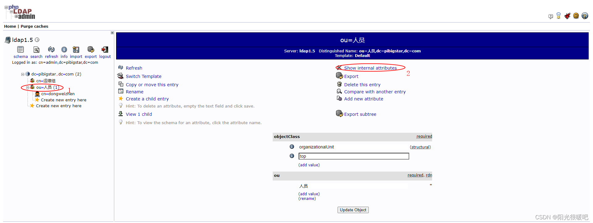
rancher集成ldap,实现统一账号登录
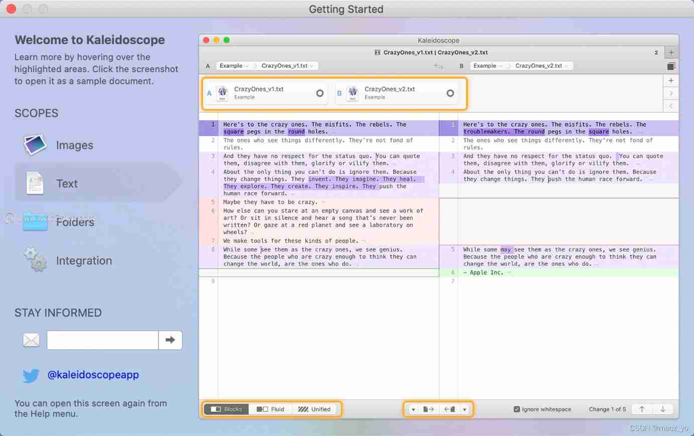
File and image comparison tool kaleidoscope latest download
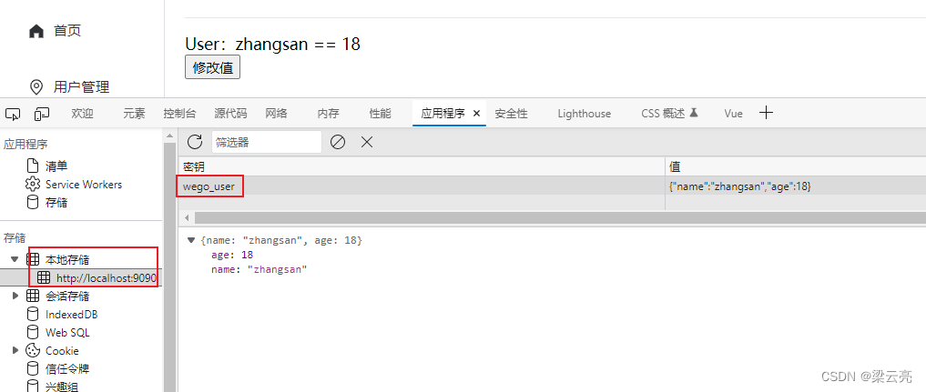
【精品】pinia 基于插件pinia-plugin-persist的 持久化

Clipboard management tool paste Chinese version
Business process testing based on functional testing
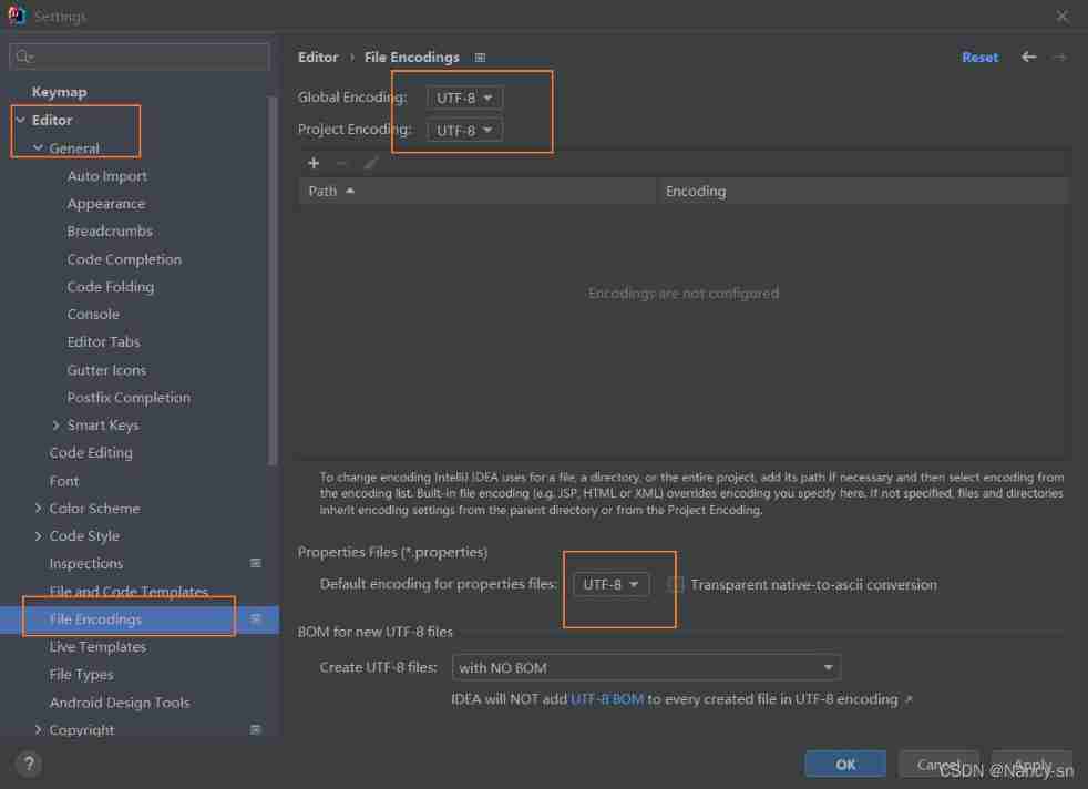
How to set encoding in idea
DAY FIVE
JWT signature does not match locally computed signature. JWT validity cannot be asserted and should
随机推荐
openresty ngx_lua子请求
[automated testing framework] what you need to know about unittest
Pinia module division
Interesting wine culture
Command line kills window process
File and image comparison tool kaleidoscope latest download
PostgreSQL uses pgpool II to realize read-write separation + load balancing
Use type aliases in typescript
Encryption algorithm - password security
St table
uniapp中redirectTo和navigateTo的区别
Leecode brush questions record sword finger offer 43 The number of occurrences of 1 in integers 1 to n
DAY TWO
After leaving a foreign company, I know what respect and compliance are
48 page digital government smart government all in one solution
【精品】pinia 基于插件pinia-plugin-persist的 持久化
Pytest multi process / multi thread execution test case
2022 PMP project management examination agile knowledge points (9)
If the college entrance examination goes well, I'm already graying out at the construction site at the moment
Rails 4 asset pipeline vendor asset images are not precompiled