当前位置:网站首页>Machine learning notes - bird species classification using machine learning
Machine learning notes - bird species classification using machine learning
2022-07-07 03:43:00 【Sit and watch the clouds rise】
One 、 Summary of problems
Scientists have determined that , A known bird should be divided into 3 Different and independent species . These species are endemic to specific areas of the country , Their populations must be tracked and estimated as accurately as possible .
therefore , A non-profit conservation association undertook this task . They need to be able to record the species they encounter based on the characteristics observed by field officials .
Use some genetic characteristics and location data , Can you predict the bird species that have been observed ?
This is a beginner level practice competition , Your goal is to predict the species of birds based on their attributes or locations .
 https://bitgrit.net/competition/16
Two 、 Data sets
The data has been easily split into training and test data sets . In every training and test , You will get a position 1 To 3 Bird data .
Dataset download address
 link :https://pan.baidu.com/s/1aalzQNr0IQLQc3X4JTu9nQ
 Extraction code :xvy0
Let's take a look at the first five lines training_set.csv
| bill_depth | bill_length | wing_length | location | mass | sex | ID |
| 14.3 | 48.2 | 210 | loc_2 | 4600 | 0 | 284 |
| 14.4 | 48.4 | 203 | loc_2 | 4625 | 0 | 101 |
| 18.4 | NA | 200 | loc_3 | 3400 | 0 | 400 |
| 14.98211382 | 47.50487805 | NA | NA | 4800 | 0 | 98 |
| 18.98211382 | 38.25930705 | 217.1869919 | loc_3 | 5200 | 0 | 103 |
training_set and training_target According to ‘id’ Column Association .
The meaning of column is as follows
species      :  Animal species  (A, B, C)
bill_length :  Beak length  (mm)
bill_depth   :  Deep beak  (mm)
wing_length :  Wing length  (mm)
mass         :  weight  (g)
location     :  Island  (Location 1, 2, 3 )
 Gender          : Animal sex (0: men ;1: women ;NA: Unknown )
3、 ... and 、 Write code
1、 Import library
import pandas as pd

# plotting
import matplotlib
import matplotlib.pyplot as plt
import seaborn as sns
matplotlib.rcParams['figure.dpi'] = 100
sns.set(rc={'figure.figsize':(11.7,8.27)})
sns.set(style="whitegrid")
%matplotlib inline

# ml
from sklearn.metrics import ConfusionMatrixDisplay, classification_report
from sklearn.model_selection import train_test_split
from sklearn.impute import SimpleImputer
from sklearn.preprocessing import LabelEncoder
from sklearn.tree import DecisionTreeClassifier
from sklearn import tree
2、 How to deal with missing values
def missing_vals(df):
    """prints out columns with perc of missing values"""
    missing = [
        (df.columns[idx], perc)
        for idx, perc in enumerate(df.isna().mean() * 100)
        if perc > 0
    ]

    if len(missing) == 0:
        return "no missing values"


    # sort desc by perc
    missing.sort(key=lambda x: x[1], reverse=True)

    print(f"There are a total of {len(missing)} variables with missing values\n")

    for tup in missing:
        print(str.ljust(f"{tup[0]:<20} => {round(tup[1], 3)}%", 1))
3、 Load data
First , We use read_csv Function to load training and test data .
We will also training_set.csv( Include features ) And training_target.csv( Contains the target variable ) Combine and form training data .
train = pd.read_csv("dataset/training_set/training_set.csv")
labels = pd.read_csv("dataset/training_set/training_target.csv")

# join target variable to training set
train = train.merge(labels, on="ID")

test = pd.read_csv("dataset/test_set/test_set.csv")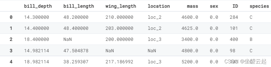
target_cols = "species"
num_cols = ["bill_depth", "bill_length", "wing_length", "mass"]
cat_cols = ["location", "sex"]
all_cols = num_cols + cat_cols + [target_cols]

train = train[all_cols]
4、 Exploratory data analysis Exploratory Data Analysis (EDA)
This is where we study data trends and patterns , Including numbers and classifications .
train.info()Use info function , We can see the number of rows and data types .
<class 'pandas.core.frame.DataFrame'>
Int64Index: 435 entries, 0 to 434
Data columns (total 7 columns):
 #   Column       Non-Null Count  Dtype
---  ------       --------------  -----
 0   bill_depth   434 non-null    float64
 1   bill_length  295 non-null    float64
 2   wing_length  298 non-null    float64
 3   mass         433 non-null    float64
 4   location     405 non-null    object
 5   sex          379 non-null    float64
 6   species      435 non-null    object
dtypes: float64(5), object(2)
memory usage: 27.2+ KB
Numerical
Let's draw a histogram of numerical variables .
train[num_cols].hist(figsize=(20, 14));
bill_depth stay 15 and 19 Peak left and right
The length of the note is 39 and 47 Peak left and right
Wings grow in 190 and 216 Peak left and right
The mass tilts to the right
Categorical
to_plot = cat_cols + [target_cols]
fig, axes = plt.subplots(1, 3, figsize=(20, 7), dpi=100)

for i, col_name in enumerate(train[to_plot].columns):
    sns.countplot(x = col_name, data = train, palette="Set1", ax=axes[i % 3])
    axes[i % 3].set_title(f"{col_name}", fontsize=13)
    plt.subplots_adjust(hspace=0.45)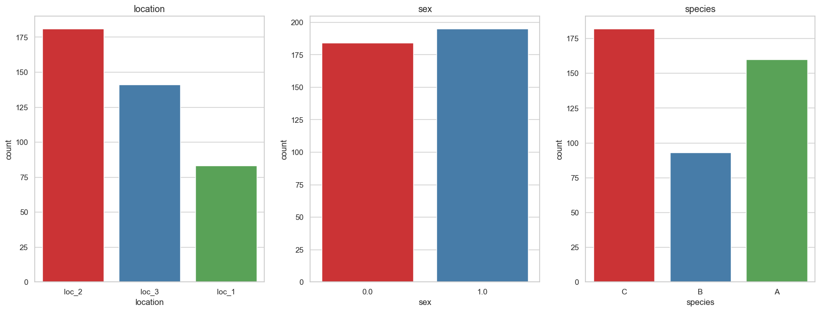
We see that the location and species seem to match their respective locations and species (loc2 And species C、loc3 And species A). We also see females (1) There are slightly more birds than males .
train.species.value_counts()C 182
A 160
B 93
Name: species, dtype: int64Observe carefully , We find that the target variable is unbalanced , among B analogy C Low near 100 Classes , Than A Low, about 70 individual .
Unbalanced classes are a problem , Because it makes the model prefer to pay more attention to classes with more samples , namely . C Than B More often predicted .
5、 missing data
Percentage of missing values
missing_vals(train)There are a total of 6 variables with missing values
bill_length => 32.184%
wing_length => 31.494%
sex => 12.874%
location => 6.897%
mass => 0.46%
bill_depth => 0.23%Through our auxiliary function , We found that bill_length and wing_length There are more than 30% The missing value
Thermogram Heatplot
plt.figure(figsize=(10, 6))
sns.heatmap(train.isnull(), yticklabels=False, cmap='viridis', cbar=False);
We can also draw heat maps to visualize missing values and see if there are any patterns .
Estimate classification column
Let's first look at how many missing variables are in our classification variables
train.sex.value_counts(dropna=False)1.0 195
0.0 184
NaN 56
Name: sex, dtype: int64train.location.value_counts(dropna=False)loc_2 181
loc_3 141
loc_1 83
NaN 30
Name: location, dtype: int64Let's use the simple imputer To deal with them , Replace them with the most frequent values .
cat_imp = SimpleImputer(strategy="most_frequent")

train[cat_cols] = cat_imp.fit_transform(train[cat_cols])
To confirm again , There are no missing values . As you can see , adopt “ Most frequent ” Strategy , The missing value is estimated as 1.0, This is the most frequent .
train.sex.value_counts(dropna=False)1.0 251
0.0 184
Name: sex, dtype: int64Estimated value column
Let's use the median to estimate our value
num_imp = SimpleImputer(strategy="median")

train[num_cols] = num_imp.fit_transform(train[num_cols])missing_vals(train)'no missing values'6、 Feature Engineering
train.species.value_counts()C 182
A 160
B 93
Name: species, dtype: int64Coding classification variables
Use label encoder , We can classify variables ( And target variables ) Code as numeric . We do this because most ML The model is not applicable to string values .
le = LabelEncoder()
le.fit(train['species'])
le_name_map = dict(zip(le.classes_, le.transform(le.classes_)))
le_name_map
{'A': 0, 'B': 1, 'C': 2}We can first fit the encoder to the variable , Then see what the mapping looks like , Then we can reverse the mapping
train['species'] = le.fit_transform(train['species'])For others with string variables ( The digital ) The column of , We also do the same coding .
for col in cat_cols:
    if train[col].dtype == "object":
        train[col] = le.fit_transform(train[col])
train.head()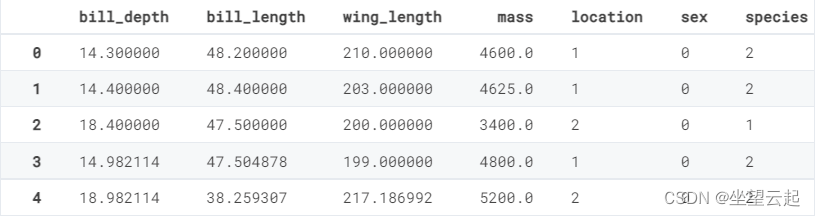
# Convert cat_features to pd.Categorical dtype
for col in cat_cols:
    train[col] = pd.Categorical(train[col])
We also transform classification features into pd.Categorical dtype
train.dtypesbill_depth float64
bill_length float64
wing_length float64
mass float64
location category
sex category
species int64
dtype: object7、 Create a new feature
train['b_depth_length_ratio'] = train['bill_depth'] / train['bill_length']
train['b_length_depth_ratio'] = train['bill_length'] / train['bill_depth']
train['w_length_mass_ratio'] = train['wing_length'] / train['mass']
ad locum , We create some features with division to form the ratio of variables
train.head()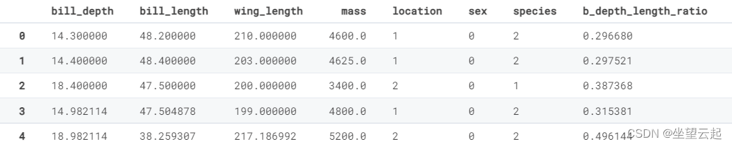
8、 Model
Training test split
Now is the time to build the model , We first split it into X( features ) and y( Target variable ), Then it is divided into training set and evaluation set .
Training is where we train our models , Evaluation is where we test the model before fitting it to the test set .
X, y = train.drop(["species"], axis=1), train[["species"]].values.flatten()

X_train, X_eval, y_train, y_eval = train_test_split(
    X, y, test_size=0.25, random_state=0)
Simple decision tree classifier
ad locum , We use max_depth = 2 Simple hyperparametric fitting baseline model
dtree_model = DecisionTreeClassifier(max_depth = 2).fit(X_train, y_train)After fitting the data , We can use it to predict
dtree_pred = dtree_model.predict(X_eval)9、 Model performance
print(classification_report(dtree_pred, y_eval)) precision recall f1-score support
0 1.00 0.70 0.82 57
1 0.71 0.92 0.80 13
2 0.75 1.00 0.86 39
accuracy 0.83 109
macro avg 0.82 0.87 0.83 109
weighted avg 0.88 0.83 0.83 109The classification report shows us the useful indicators of the classifier .
for example , We model f1-score by 0.83
10、 Confusion matrix
We can also build a confusion matrix to visualize what our classifier is doing well / bad .
# save the target variable classes
class_names = le_name_map.keys()

titles_options = [
    ("Confusion matrix, without normalization", None),
    ("Normalized confusion matrix", "true"),
]
for title, normalize in titles_options:
    fig, ax = plt.subplots(figsize=(8, 8))

    disp = ConfusionMatrixDisplay.from_estimator(
        dtree_model,
        X_eval,
        y_eval,
        display_labels=class_names,
        cmap=plt.cm.Blues,
        normalize=normalize,
        ax = ax
    )
    disp.ax_.set_title(title)
    disp.ax_.grid(False)

    print(title)
    print(disp.confusion_matrix)
Confusion matrix, without normalization
[[40 0 0]
[ 5 12 0]
[12 1 39]]
Normalized confusion matrix
[[1. 0. 0. ]
[0.29411765 0.70588235 0. ]
[0.23076923 0.01923077 0.75 ]]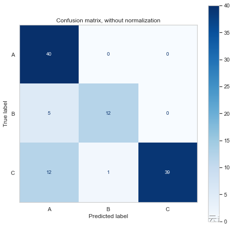
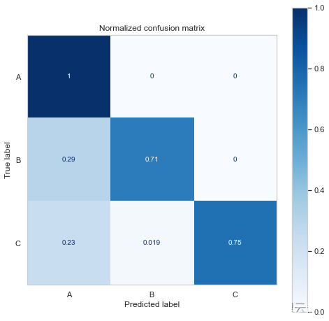
The confusion matrix shows us that it predicts more A Classes and C class , That's not surprising , Because we have more samples .
It also shows that the model should be B/C I predicted more A class .
11、 Importance of features
feature_imp = pd.DataFrame(sorted(zip(dtree_model.feature_importances_,X.columns)), columns=['Value','Feature'])

plt.figure(figsize=(20, 15))
sns.barplot(x="Value", y="Feature", data=feature_imp.sort_values(by="Value", ascending=False))
plt.title('LightGBM Features')
plt.tight_layout()
# plt.savefig('lightgbm_fimp.png')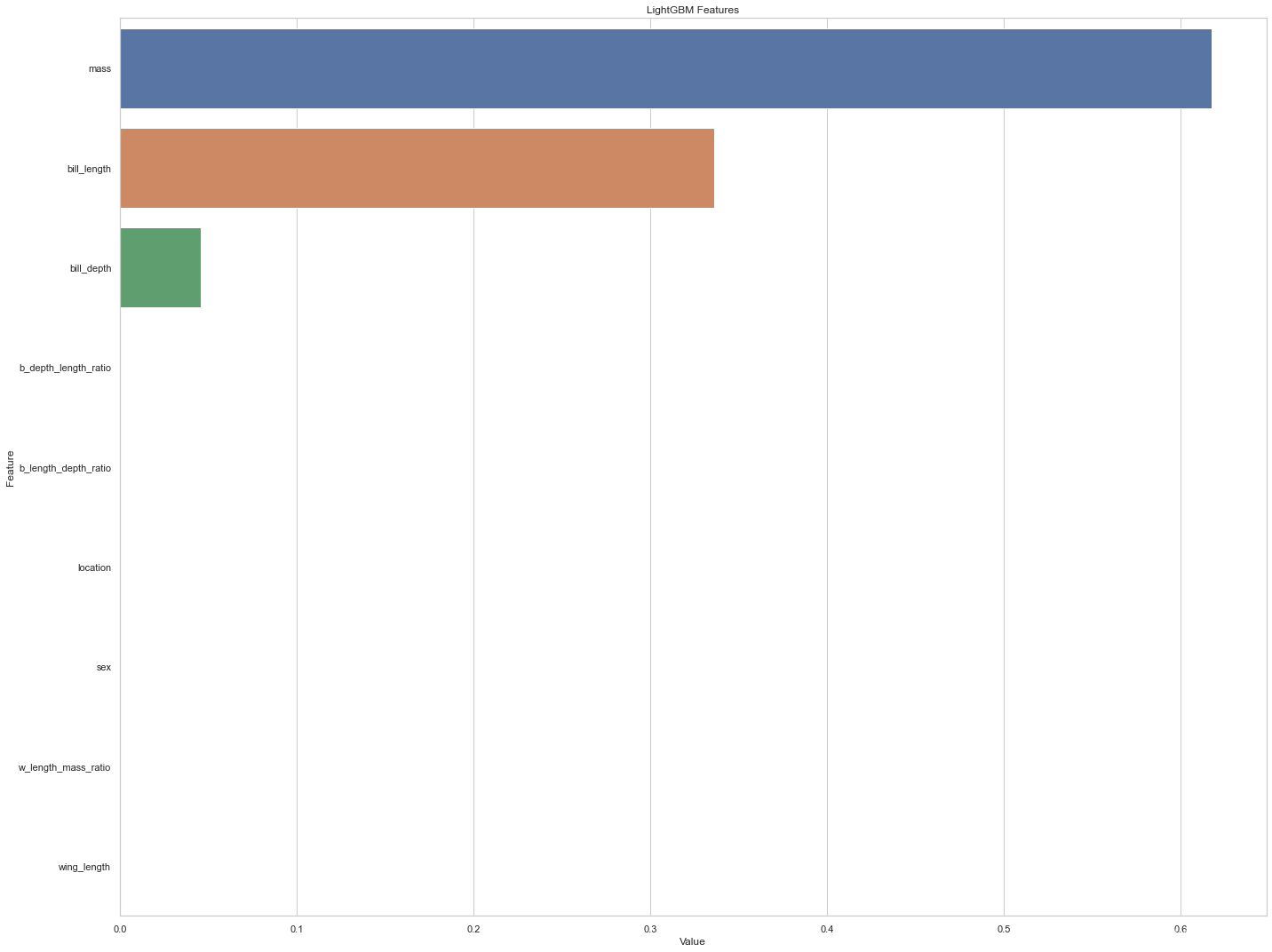
In terms of the importance of characteristics , It seems that quality has the best ability to predict species , Secondly, the beak is long . The importance of other variables in the classifier seems to be zero
fig = plt.figure(figsize=(25,20))
_ = tree.plot_tree(dtree_model,
                   feature_names=X.columns,
                   class_names=list(class_names),
                   filled=True)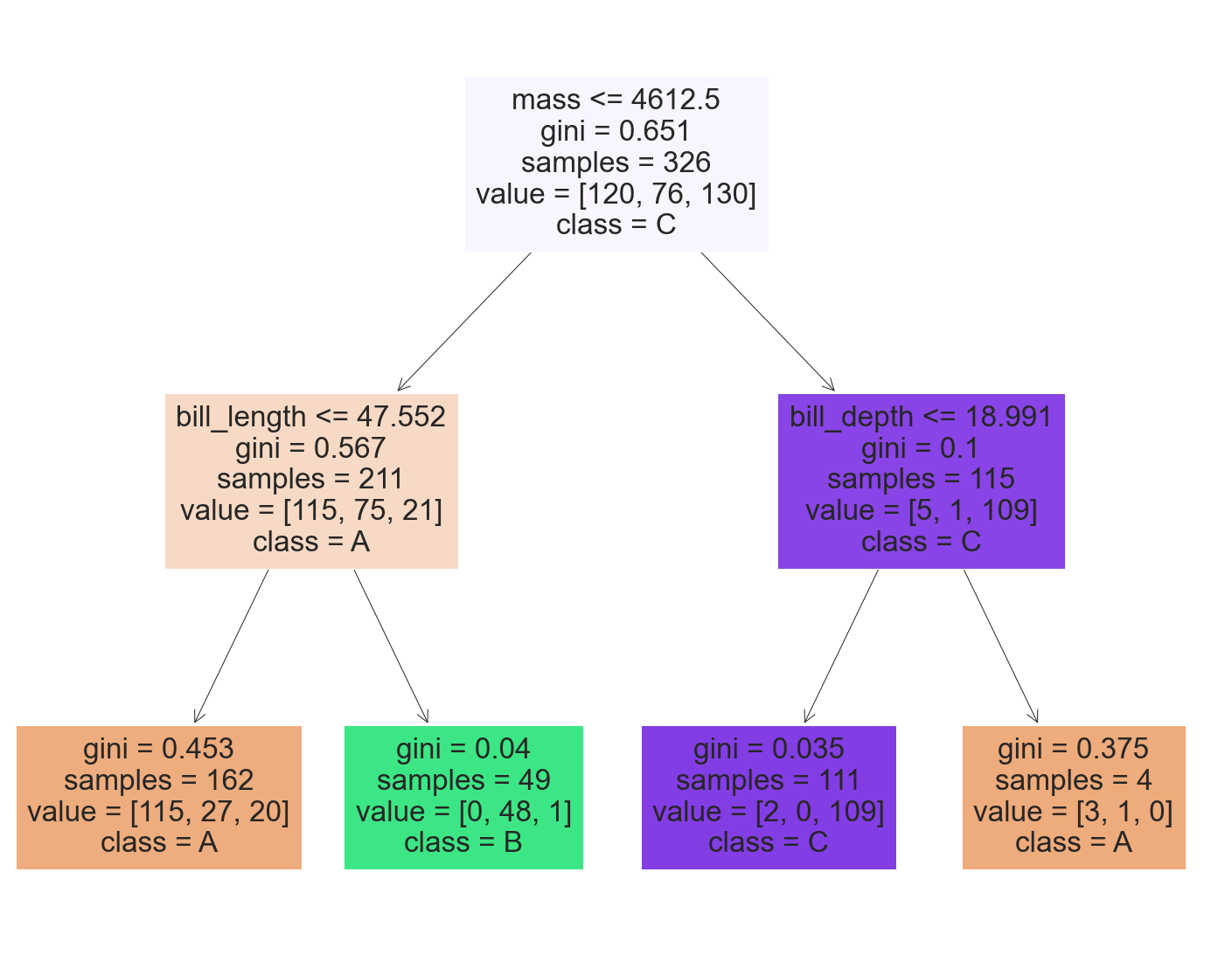
We saw how to use feature importance in the visualization of our decision tree classifier .
In the root node , If the quality is lower than 4600 about , Then check bill_length, Otherwise check bill_depth, Then predict the category at the leaf .
Four 、 Forecast test data
Now is the time before we fit the model to the test data , The same feature preprocessing and engineering are carried out on the training data .
le = LabelEncoder()

cat_imp = SimpleImputer(strategy="most_frequent")
num_imp = SimpleImputer(strategy="median")

test[cat_cols] = cat_imp.fit_transform(test[cat_cols])
test[num_cols] = num_imp.fit_transform(test[num_cols])

for col in cat_cols:
    if test[col].dtype == "object":
        test[col] = le.fit_transform(test[col])

# Convert cat_features to pd.Categorical dtype
for col in cat_cols:
    test[col] = pd.Categorical(test[col])

# save ID column
test_id = test["ID"]

all_cols.remove('species')
test = test[all_cols]

test['b_depth_length_ratio'] = test['bill_depth'] / test['bill_length']
test['b_length_depth_ratio'] = test['bill_length'] / test['bill_depth']
test['w_length_mass_ratio'] = test['wing_length'] / test['mass']
test_preds = dtree_model.predict(test)
submission_df = pd.concat([test_id, pd.DataFrame(test_preds, columns=['species'])], axis=1)
submission_df.head()| ID | species | |
|---|---|---|
| 0 | 2 | 2 |
| 1 | 5 | 0 |
| 2 | 7 | 0 |
| 3 | 8 | 0 |
| 4 | 9 | 0 |
Please note that , Species values are numbers , We have to convert it back to a string value . Use with fit Tag encoder , We can do that .
le_name_map{'A': 0, 'B': 1, 'C': 2}inv_map = {v: k for k, v in le_name_map.items()}
inv_map{0: 'A', 1: 'B', 2: 'C'}submission_df['species'] = submission_df['species'].map(inv_map)
submission_df.head()| ID | species | |
|---|---|---|
| 0 | 2 | C |
| 1 | 5 | A |
| 2 | 7 | A |
| 3 | 8 | A |
| 4 | 9 | A |
submission_df.to_csv('solution.csv', index=False)Last , We write the data frame csv file .
边栏推荐
- 维护万星开源向量数据库是什么体验
- Set static IP for raspberry pie
- 19. (ArcGIS API for JS) ArcGIS API for JS line acquisition (sketchviewmodel)
- codeforces每日5题(均1700)-第七天
- First understand the principle of network
- My brave way to line -- elaborate on what happens when the browser enters the URL
- 树莓派设置静态ip
- The latest 2022 review of "small sample deep learning image recognition"
- Stored procedures and functions (MySQL)
- Optimization cases of complex factor calculation: deep imbalance, buying and selling pressure index, volatility calculation
猜你喜欢
R data analysis: how to predict Cox model and reproduce high score articles
如何自定义Latex停止运行的快捷键
VHDL implementation of arbitrary size matrix addition operation
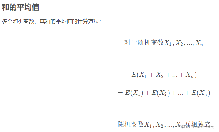
Probability formula

Experience design details

Introduction to opensea platform developed by NFT trading platform (I)
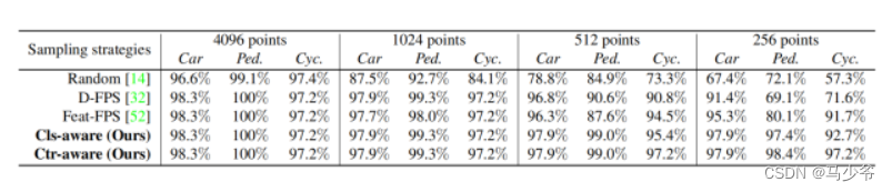
Not All Points Are Equal Learning Highly Efficient Point-based Detectors for 3D LiDAR Point
Enumeration general interface & enumeration usage specification
R数据分析:cox模型如何做预测,高分文章复现
Open3d mesh filtering
随机推荐
C# Task拓展方法
Clock in during winter vacation
Appx code signing Guide
Not All Points Are Equal Learning Highly Efficient Point-based Detectors for 3D LiDAR Point
Hisilicon 3559 universal platform construction: RTSP real-time playback support
Construction of Hisilicon universal platform: color space conversion YUV2RGB
R数据分析:cox模型如何做预测,高分文章复现
海思3559万能平台搭建:RTSP实时播放的支持
Optimization cases of complex factor calculation: deep imbalance, buying and selling pressure index, volatility calculation
源代码保密的意义和措施
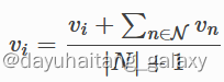
卡尔曼滤波-1
The latest 2022 review of "small sample deep learning image recognition"
树莓派设置静态ip
【DPDK】dpdk样例源码解析之三:dpdk-l3fwd_001
本机mysql
Kalman filter-1
Function reentry, function overloading and function rewriting are understood by yourself
Baidu map JS development, open a blank, bmapgl is not defined, err_ FILE_ NOT_ FOUND
Leetcode-02 (linked list question)
我的勇敢对线之路--详细阐述,浏览器输入URL发生了什么