当前位置:网站首页>Matplotlib swordsman - a stylist who can draw without tools and code
Matplotlib swordsman - a stylist who can draw without tools and code
2022-07-02 09:13:00 【Qigui】
Individuality signature : The most important part of the whole building is the foundation , The foundation is unstable , The earth trembled and the mountains swayed . And to learn technology, we should lay a solid foundation , Pay attention to me , Take you to firm the foundation of the neighborhood of each plate .
Blog home page : Qigui's blog
Included column :Python The Jianghu cloud of the three swordsmen
From the south to the North , Don't miss it , Miss this article ,“ wonderful ” May miss you yo
Triple attack( Three strikes in a row ):Comment,Like and Collect—>Attention
List of articles
Write it at the front
Trilogy on the eve of painting
canvas
- adopt plt.figure To create a canvas ——plt.figure(figsize(a,b), facecolor=‘r’)
Change Chinese font
- Matplotlib Encountered the problem of Chinese display box in
- adopt plt.rcParams[‘font.sans-serif’] = ‘Microsoft YaHei’ solve
- The Chinese fonts that can be set are SimSun( Song style ),SimHei( In black ),Kaiti( Regular script ) etc.
Negative signs show problems
- adopt plt.rcParams[‘axes.unicode_minus’] = False solve
Stylist —— Style parameters
Most drawing methods have style options , Can access the current call drawing method , Or from Artist Upper “setter” call . In the inside picture , We set it manually Color 、 Lineweight and linetype plot, We set the linetype of the second line to call set_linestyle.
import numpy as np
import matplotlib.pyplot as plt

#  Load Fonts
plt.rcParams['font.sans-serif'] = ['SimHei']  #  Specify default font
#  Show minus sign
plt.rcParams['axes.unicode_minus'] = False

data1, data2, data3, data4 = np.random.randn(4, 150)  #  establish 4 A random data set

fig, ax = plt.subplots(figsize=(10, 6))
x = np.arange(len(data1))
ax.plot(x, np.cumsum(data1), color='g', linewidth=4, linestyle='--')
l, = ax.plot(x, np.cumsum(data2), color='b', linewidth=3)	#  This is called set_linestyle
l.set_linestyle(':')
plt.show()
Output graph :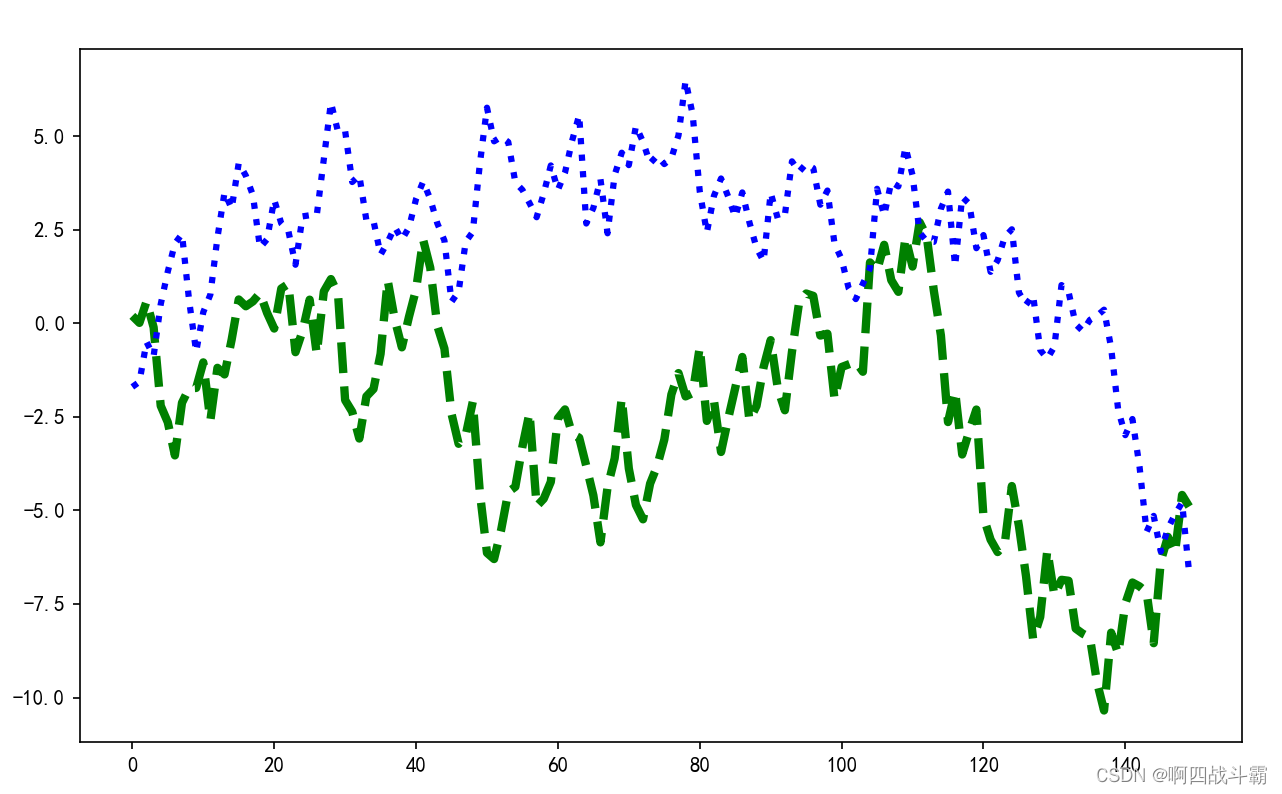
Color
Matplotlib There is a very flexible color array , Will use a variety of colors . That is, for a scatter mapping , The edge and interior of the mark can be different colors :
- color—— Assign colors
- alpha(0-1)—— transparency
- colormap—— Color board
data1, data2, data3, data4 = np.random.randn(4, 150)  #  establish 4 A random data set
x = np.arange(len(data1))

fig, ax = plt.subplots(figsize=(10, 6))
ax.scatter(data1, data2, s=50, facecolor='b', edgecolor='r')	#  The edge color of the mark is red , The interior color is blue
plt.show()
Output graph :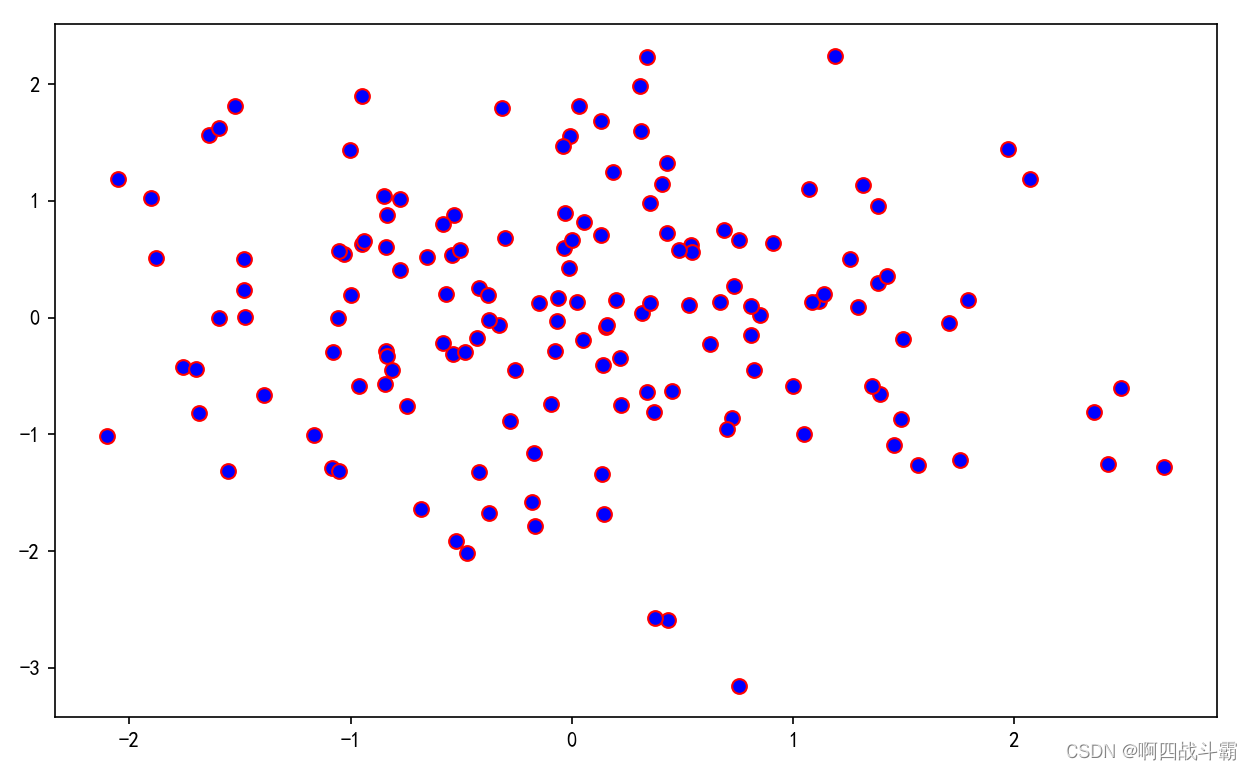
linear
- linewidth—— Line width , It can be abbreviated as :’lw‘, Set the thickness of the line
- linestyle—— Linetype
Mark
marker—— Mark
markerwidth—— Tag size
Unfilled tags

Fill mark

fig, ax = plt.subplots(figsize=(10, 6))
ax.plot(data1, 'o', label='data1')
ax.plot(data2, 'd', label='data2')
ax.plot(data3, 'v', label='data3')
ax.plot(data4, 's', label='data4')
ax.legend()
plt.show()
Output graph :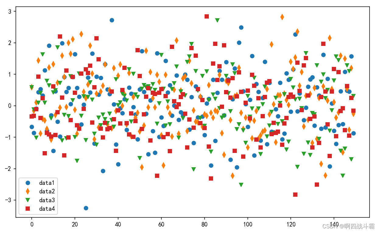
- style Parameters , Can contain linestyle,marker,color
import pandas as pd
import numpy as np

# style Parameters , Can contain linestyle,marker,color

ts = pd.Series(np.random.randn(1000).cumsum(), index=pd.date_range('1/1/2000', periods=1000))
ts.plot(style='--g.')
# style →  Style string , This includes linestyle(-),marker(.),color(g)
plt.show()
Output graph :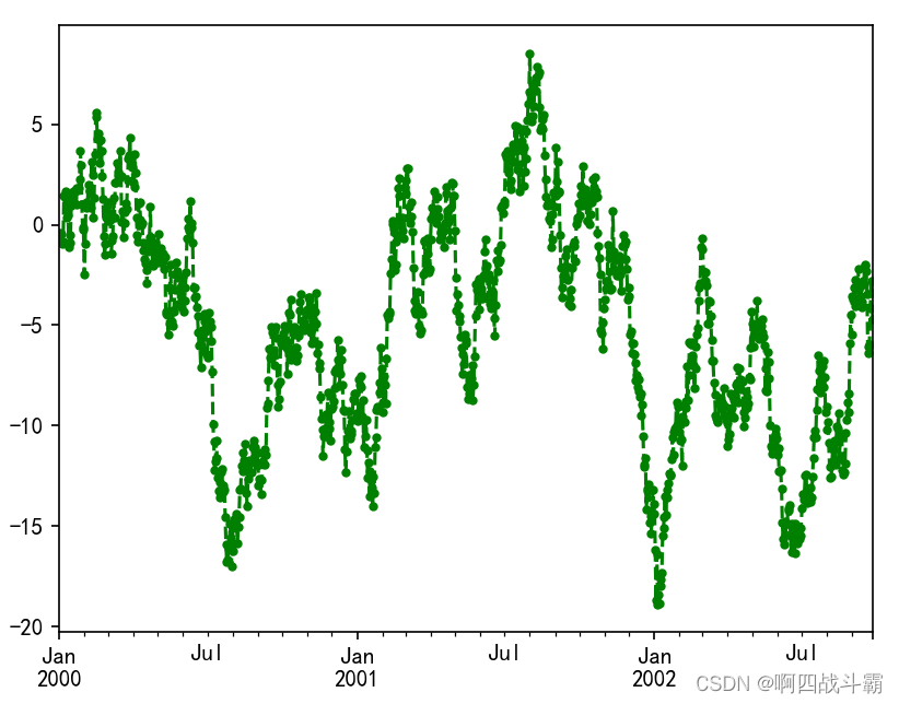
Mark parcels —— The basic elements
Axis labels and text
- set_xlabel, set_ylabel, and set_title Used to add text at the specified position
- Text can also be used directly text Add to drawing
Add chart title
- adopt plt.title Can be in Matplotlib Set title
- Font styles can be created by fontdict Set it up
- fontsize—— Set the title size
- adopt loc Parameter can set the title display position , The supported parameters are :
- center( In the middle )
- left( Keep to the left )
- right( Keep right )
Add axis title
- Add axis title
- adopt plt.xlabel and plt.ylabel You can add... Separately x Axis and y The title of the axis
- It can also be done by fontdict Configure font styles
- fontsize—— Set the title size
- labelpad You can set the distance between the coordinate axis and the title
Add data label ——text
Can pass plt.text Add text to the chart , But only one point can be added at a time , So if you want to add labels to every data item , We need to pass for loop To carry out
- plt.text There are three important parameters :
- x、y 、s, adopt x and y Determine the display position ,s For the text that needs to be displayed
- And then there is va and ha Two parameters set the display position of the text ( Keep to the left 、 Keep right 、 Center, etc )
- Spaces require —— Transfer characters \
- fontdict—— Set the size and color of text words , Need to use dict Form into
mu, sigma = 120, 20
x = mu + sigma * np.random.randn(1000)
fig, ax = plt.subplots(figsize=(10, 6))
#  Histogram of data
n, bins, patches = ax.hist(x, 50, density=1, facecolor='C0', alpha=0.75)

ax.set_xlabel('Length [cm]')    # x Axis labels
ax.set_ylabel('Probability')    # y Axis labels
ax.set_title('Aardvark lengths\n (not really)')     #  title
#  ad locum  r  Before the title string, it means that the string is   original   character string , Instead of treating backslashes as  python  escape
ax.text(75, .025, r'$\mu=120,\ \sigma=20$')     #  To add text —— Here is the use of mathematical expressions in text
ax.axis([55, 175, 0, 0.03])
ax.grid(True)   #  Adding grid
plt.show()
Output graph :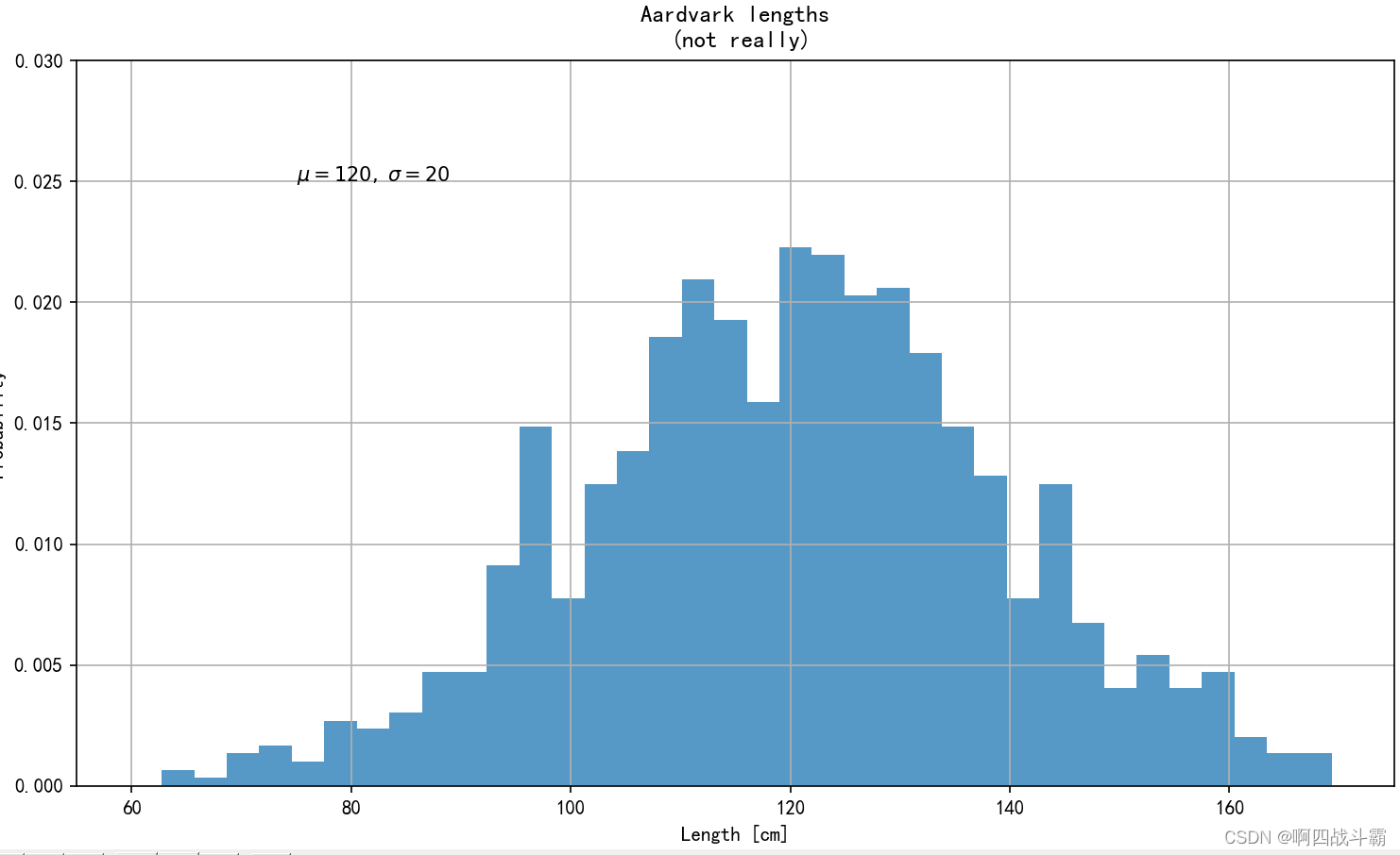
notes —— To add text annotate
You can also mark points on the figure , Usually by connecting arrows xytext Point to xy
annotate() Basic use
- text—— It's the text of the comment
- xy—— It's the coordinates of the points that need to be annotated , Used to locate the position to be marked
- xytext—— Is the coordinates of the annotation text ( Mark the location ), Prompt the position of the text to be displayed
- arrowprops—— It is the setting of arrow type and arrow radian in the figure , Need to use dict Form into
- xycoords=‘data’—— Choose a location based on the value of the data , Set up xy How to locate , such as data Indicates that the coordinate axis scale value is used for positioning
- textcoords=‘offset points’——xy Deviation value , Same as xycoords, Set up xytext How to locate
t = np.arange(0.0, 5.0, 0.01)
s = np.cos(2 * np.pi * t)

fig, ax = plt.subplots(figsize=(10, 6))
line, = ax.plot(t, s, linewidth=2)
ax.annotate('local max', xy=(2, 1), xytext=(3, 1.5),
            arrowprops=dict(facecolor='black', shrink=0.05))

ax.set_ylim(-2, 2)
plt.show()
Output graph :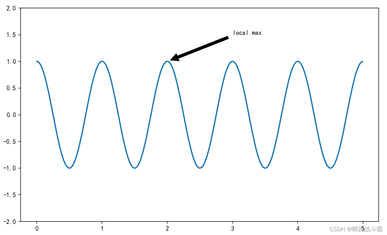
Legend has it that —— legend legend
adopt plt.legend You can add a legend to the chart , The legend is usually used to explain the data of each series in the chart
- legend—— Show Legend
- fontsize—— Set font size
- By setting handles Parameter to select the content displayed in the legend
- loc—— Indicate location
- ‘best’ : 0 ( Adaptive way )
- ‘upper right’ : 1
- ‘upper left’ : 2
- ‘lower left’ : 3
- ‘lower right’ : 4
- ‘right’ : 5
- ‘center left’ : 6
- ‘center right’ : 7
- ‘lower center’ : 8
- ‘upper center’ : 9
- ‘center’ : 10
data1, data2, data3 = np.random.randn(3, 150)  #  establish 3 A random data set
x = np.arange(len(data1))

fig, ax = plt.subplots(figsize=(10, 6))
ax.plot(np.arange(len(data1)), data1, label='data1')
ax.plot(np.arange(len(data2)), data2, label='data2')
ax.plot(np.arange(len(data3)), data3, 'd', label='data3')
ax.legend(loc='best')     #  Add legend
plt.show()
Output graph :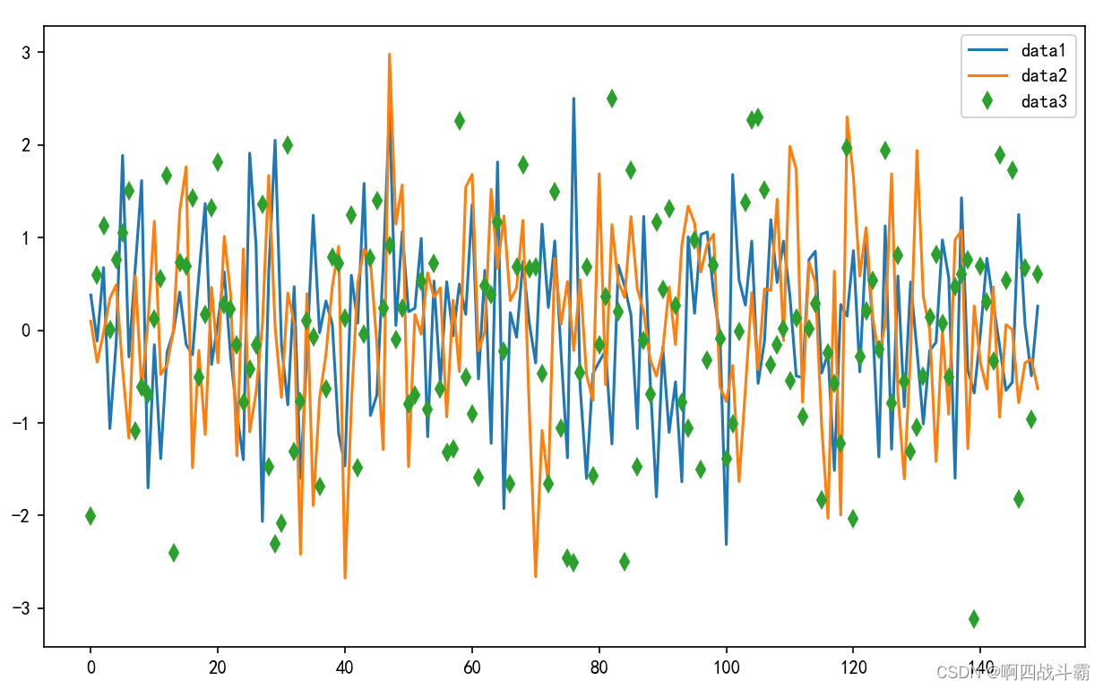
Add grid lines ——grid
By adding grid lines, users can easily see the approximate value of data items , When displaying all data labels through the above , It may make the whole chart more messy , We can choose to use gridlines to show the approximate data values of data items
Parameters b by True Show gridlines when
axis Support x、y、both Three values , respectively
- x—— Vertical gridlines
- y—— Horizontal gridlines
- both—— Vertical and horizontal
Other linetype configurations are similar to the parameters of configuring polyline style , Such as : Linetype 、 Line width 、 Color
Leave the canvas blank ——tight_layout()
Because the chart and Figure Insufficient white space , The legend cannot be displayed completely .Matplotlib Inside the module tight_layout() function , Settings are available pad Parameters are shown in the chart and Figure Set a blank space between ( There is no need to set pad Parameters )
- plt.tight_layout()—— Tighten the space around , Expand the usable area of the drawing area
- h_pad /v_pad You can set the height separately / Width blank
Shaft scale and scale
- tick params()—— Set axis :
- Scale size (labelsize)
- ( Scale line ) Color (color)
- Range of application (axis)
- tick_params(axis=‘xx’,labelsize=b,color=‘r’)
- labelsize Of b Represents the scale size
- If axis Of xx yes both Represents the application to x and y Axis , If xx yes x Represents the application to x Axis , If xx yes y Represents the application to y Axis .
- color Is to set the line color of the scale , for example ,red For red
x = np.linspace(-3, 3, 50)
y1 = 2 * x + 1
y2 = x ** 2

plt.figure(num=3, figsize=(8, 5))
plt.plot(x, y2)
plt.plot(x, y1, color='red', linewidth=1.0, linestyle='--')
plt.tick_params(axis='both', labelsize=18, color='red')
plt.show()
Output graph :
Coordinate range and axis scale
occasionally , Our axis scale may not be a series of numbers , But some words , Or we want to adjust the sparsity of the scale of the coordinate axis
At this time , You need to use plt.xticks() perhaps plt.yticks() To adjust : First , Use np.linspace Define the new scale range and number : The scope is (-1,2); The number is 5.
- plt.axis—— Simultaneous setting x,y Axis coordinate range
- plt.xlim—— Set up x Axis range :(-1, 2)
- plt.ylim—— Set up y Axis range :(-2, 3)
- plt.xticks—— Set up x Axis scale and name : The scope is (-1,2); The number is 5.
- plt.yticks—— Set up y Axis scale and name : Scale is [-2, -1.8, -1, 1.22, 3]; The name of the corresponding scale is [‘really bad’,’bad’,’normal’,’good’, ‘really good’].
x = np.linspace(-3, 3, 50)
y1 = 2 * x + 1
y2 = x ** 2

plt.figure(num=3, figsize=(8, 5))
plt.plot(x, y2)
plt.plot(x, y1, color='red', linewidth=1.0, linestyle='--')

plt.axis([-1, 2, -2, 3])	#  Use  axis() Set up x,y The minimum and maximum scales of the shaft
plt.xlim((-1, 2))  # x Axis coordinate range
plt.ylim((-2, 3))  # y Axis coordinate range

new_ticks = np.linspace(-1, 2, 5)
plt.xticks(new_ticks)  # x Axis scale ( You can also set the name here, such as bar chart )
plt.yticks([-2, -1.8, -1, 1.22, 3], [r'$really\ bad$', r'$bad$', r'$normal$', r'$good$', r'$really\ good$'])  # y Shaft scale and name
plt.show()
Output graph :
Adjust the scale and border position
- Use .xaxis.set_ticks_position Set up x The position of a coordinate scale number or name :
- bottom.( All positions :top,bottom,both,default,none)
- Use .spines Set borders :x Axis ; Use .set_position Set border position :y=0 The location of ;( Position all attributes :outward,axes,data)
The code is as follows :
ax.xaxis.set_ticks_position('bottom')
ax.spines['bottom'].set_position(('data', 0))
figure :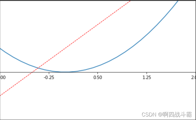
- Use .yaxis.set_ticks_position Set up y The position of a coordinate scale number or name :
- left.( All positions :left,right,both,default,none)
- Use .spines Set borders :y Axis ; Use .set_position Set border position :x=0 The location of ;( Position all attributes :outward,axes,data)
The code is as follows :
ax.yaxis.set_ticks_position('left')
ax.spines['left'].set_position(('data',0))
figure :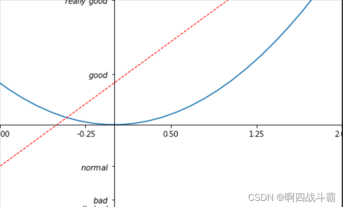
Set the image border color
Careful partners may notice , Our image coordinate axis is always composed of four lines up, down, left, right , We can also modify them :
- plt.gca()—— Get the current axis information
- Use .spines—— Set borders : Right border
- Use .set_color—— Set border color : Default white
- Use .spines Set borders : On the border
- Use .set_color Set border color : Default white
The code is as follows :
ax = plt.gca()
ax.spines['right'].set_color('none')
ax.spines['top'].set_color('none')
In the last
After reading the knowledge points , It's your turn to pass “ Stylist ” I'm addicted to it . Interested partners can combine the above learning , Do it yourself , Only in this way can we firmly remember !
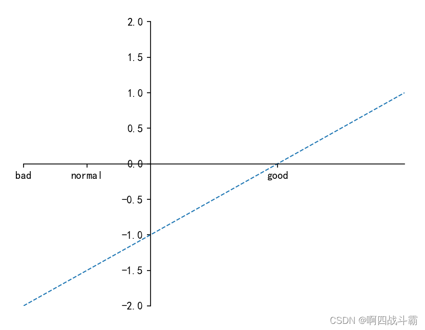
One :
Draw a straight line y = x-1, The line type is dashed , The line width is 1, The ordinate range (-2,1), The abscissa range (-1,2), The horizontal and vertical coordinates are (0,0) Coordinate points intersect . In abscissa [-1,-0.5,1] They correspond to each other [bad, normal, good]
- Result chart :
Two :
x = [‘1 month ’, ‘2 month ’, ‘3 month ’, ‘4 month ’, ‘5 month ’, ‘6 month ’, ‘7 month ’, ‘8 month ’, ‘9 month ’, ‘10 month ’, ‘11 month ’, ‘12 month ’]
y = [123, 145, 152, 182, 147, 138, 189, 201, 203, 211, 201, 182]
requirement :
1. The line type and marked points are shown in the figure , You can refer to this chapter to find the corresponding code
2. The color is set to rgba(255, 0, 0, 0.5)
3. The line width is 2, The marking size is 15
- Result chart :

边栏推荐
- Knowledge points are very detailed (code is annotated) number structure (C language) -- Chapter 3, stack and queue
- Microservice practice | declarative service invocation openfeign practice
- CSDN Q & A_ Evaluation
- Gocv image reading and display
- I've taken it. MySQL table 500W rows, but someone doesn't partition it?
- Using recursive functions to solve the inverse problem of strings
- Watermelon book -- Chapter 6 Support vector machine (SVM)
- 破茧|一文说透什么是真正的云原生
- 我服了,MySQL表500W行,居然有人不做分区?
- AMQ6126问题解决思路
猜你喜欢
2022/2/13 summary
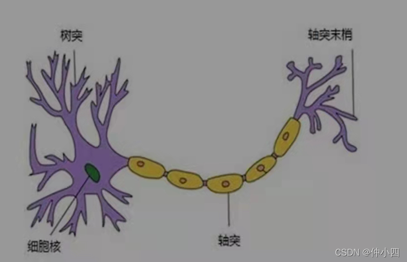
Watermelon book -- Chapter 5 neural network

Avoid breaking changes caused by modifying constructor input parameters
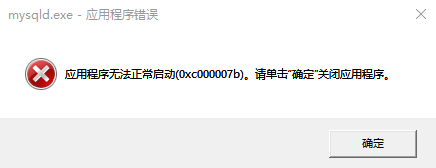
Mysql安装时mysqld.exe报`应用程序无法正常启动(0xc000007b)`
【Go实战基础】如何安装和使用 gin
![[go practical basis] how can gin get the request parameters of get and post](/img/fd/66074d157d93bcf20a5d3b37da9b3e.png)
[go practical basis] how can gin get the request parameters of get and post

Chrome视频下载插件–Video Downloader for Chrome
![[go practical basis] how to customize and use a middleware in gin](/img/fb/c0a4453b5d3fda845c207c0cb928ae.png)
[go practical basis] how to customize and use a middleware in gin
查看was发布的应用程序的端口

洞见云原生|微服务及微服务架构浅析
随机推荐
C nail development: obtain all employee address books and send work notices
Redis安装部署(Windows/Linux)
2022/2/13 summary
Matplotlib swordsman Tour - an artist tutorial to accommodate all rivers
Solution and analysis of Hanoi Tower problem
Multi version concurrency control mvcc of MySQL
Oracle 相关统计
Move a string of numbers backward in sequence
西瓜书--第五章.神经网络
「Redis源码系列」关于源码阅读的学习与思考
2022/2/14 summary
微服务实战|手把手教你开发负载均衡组件
C# 将网页保存为图片(利用WebBrowser)
[staff] common symbols of staff (Hualian clef | treble clef | bass clef | rest | bar line)
Cloud computing in my eyes - PAAS (platform as a service)
[go practical basis] how to bind and use URL parameters in gin
Watermelon book -- Chapter 5 neural network
十年開發經驗的程序員告訴你,你還缺少哪些核心競爭力?
Gocv image cutting and display
Solution of Xiaomi TV's inability to access computer shared files