当前位置:网站首页>Image hyperspectral experiment: srcnn/fsrcnn
Image hyperspectral experiment: srcnn/fsrcnn
2022-07-05 12:11:00 【Hua Weiyun】
Image super-resolution is super-resolution , Change the image from blurred to clear . This paper deals with BSDS500 The data set is used for hyperspectral experiments . Complete source code file / See the end of the text for the data set acquisition method
1. The goal of the experiment
The input size is h×w Image X, Output as a sh×sw Image Y,s Is the magnification .
2. Data set profile
This experiment uses BSDS500 Data sets , The training set contains 200 Zhang image , The validation set contains 100 Zhang image , The test set contains 200 Zhang image .
Data set source :https://download.csdn.net/download/weixin_42028424/11045313
3. Data preprocessing
Data preprocessing consists of two steps :
(1) Convert picture to YCbCr Pattern
because RGB Color mode hue 、 chroma 、 Saturation is difficult to separate when the three are mixed together , So convert it into YcbCr Color mode ,Y Is the luminance component ,Cb Express RGB The blue part of the input signal and RGB The difference between signal brightness values ,Cr Express RGB The red part of the input signal and RGB The difference between signal brightness values .
(2) Cut the picture into 300×300 The square of
Because the neural network input image used later requires the same length and width , and BSDS500 The length and width of the pictures in the dataset are not consistent , Therefore, it needs to be cut . The method used here is to locate the center of each picture first , Then take the center of the picture as the benchmark , Expand in four directions 150 Pixel , To crop the picture into 300×300 The square of .
Related codes :
def is_image_file(filename): return any(filename.endswith(extension) for extension in [".png", ".jpg", ".jpeg"])def load_img(filepath): img = Image.open(filepath).convert('YCbCr') y, _, _ = img.split() return yCROP_SIZE = 300class DatasetFromFolder(Dataset): def __init__(self, image_dir, zoom_factor): super(DatasetFromFolder, self).__init__() self.image_filenames = [join(image_dir, x) for x in listdir(image_dir) if is_image_file(x)] crop_size = CROP_SIZE - (CROP_SIZE % zoom_factor) # Cut from the center of the picture into 300*300 self.input_transform = transforms.Compose([transforms.CenterCrop(crop_size), transforms.Resize( crop_size // zoom_factor), transforms.Resize( crop_size, interpolation=Image.BICUBIC), # BICUBIC Bicubic interpolation transforms.ToTensor()]) self.target_transform = transforms.Compose( [transforms.CenterCrop(crop_size), transforms.ToTensor()]) def __getitem__(self, index): input = load_img(self.image_filenames[index]) target = input.copy() input = self.input_transform(input) target = self.target_transform(target) return input, target def __len__(self): return len(self.image_filenames)4. Network structure
This experiment tried SRCNN and FSRCNN Two networks .
4.1 SRCNN
SRCNN from 2014 year Chao Dong And so on , It is the first work of deep learning in the field of image hypersegmentation . The network structure is shown in the figure below :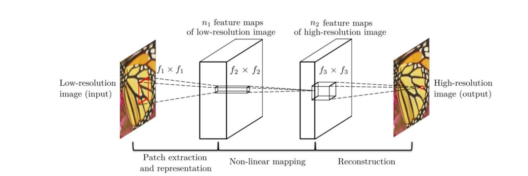
The network for a low resolution image , First, use bicubic interpolation to enlarge it to the target size , Then do nonlinear mapping through three-layer convolution network , The result obtained is output as a high-resolution image .
The author's explanation of the three convolution layers :
(1) Feature block extraction and representation : This operation starts from a low resolution image Y Extract overlapping feature blocks , Each feature block is represented as a high-dimensional vector . These vectors consist of a set of characteristic graphs , Its number is equal to the dimension of the vector .
(2) Nonlinear mapping : This operation nonlinearly maps each high-dimensional vector to another high-dimensional vector . Each mapping vector is conceptually the representation of high-resolution feature blocks . These vectors also include another set of characteristic graphs .
(3) The reconstruction : This operation aggregates the above high resolution patch-wise( An area between the pixel level and the image level ) Express , Generate the final high resolution image .
Each layer structure :
- Input : Processed low resolution image
- Convolution layer 1: use 9×9 Convolution kernel
- Convolution layer 2: use 1×1 Convolution kernel
- Convolution layer 3: use 5×5 Convolution kernel
- Output : High resolution image
Model structure code :
class SRCNN(nn.Module): def __init__(self, upscale_factor): super(SRCNN, self).__init__() self.relu = nn.ReLU() self.conv1 = nn.Conv2d(1, 64, kernel_size=5, stride=1, padding=2) self.conv2 = nn.Conv2d(64, 64, kernel_size=3, stride=1, padding=1) self.conv3 = nn.Conv2d(64, 32, kernel_size=3, stride=1, padding=1) self.conv4 = nn.Conv2d(32, upscale_factor ** 2, kernel_size=3, stride=1, padding=1) self.pixel_shuffle = nn.PixelShuffle(upscale_factor) self._initialize_weights() def _initialize_weights(self): init.orthogonal_(self.conv1.weight, init.calculate_gain('relu')) init.orthogonal_(self.conv2.weight, init.calculate_gain('relu')) init.orthogonal_(self.conv3.weight, init.calculate_gain('relu')) init.orthogonal_(self.conv4.weight) def forward(self, x): x = self.conv1(x) x = self.relu(x) x = self.conv2(x) x = self.relu(x) x = self.conv3(x) x = self.relu(x) x = self.conv4(x) x = self.pixel_shuffle(x) return x4.2 FSRCNN
FSRCNN from 2016 year Chao Dong And so on , And SRCNN Is the same author . The network structure is shown in the figure below :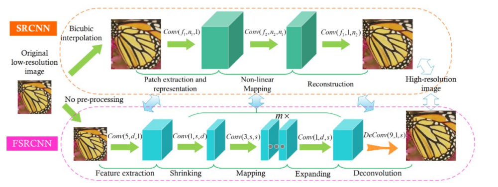
FSRCNN stay SRCNN On this basis, the following changes have been made :
1.FSRCNN The low resolution image is directly used as the input , differ SRCNN The low resolution image needs to be interpolated by bicubic interpolation first, and then used as input ;
2.FSRCNN At the end of the network, the deconvolution layer is used to realize up sampling ;
3.FSRCNN There is no nonlinear mapping in , There is a corresponding contraction 、 Mapping and extension ;
4.FSRCNN Choose smaller filters and deeper network structures .
Each layer structure :
- Input layer :FSRCNN Don't use bicubic Interpolation to upsample the input image , It goes directly into the feature extraction layer
- Feature extraction layer : use 1 × d × ( 5 × 5 ) Convolution layer extraction
- Shrinkage layer : use d × s × ( 1 × 1 ) Convolution layer to reduce the number of channels , To reduce the complexity of the model
- Mapping layer : use s × s × ( 3 × 3 ) The convolution layer is used to increase the nonlinearity of the model LR → SR Mapping
- Expansion layer : The layer and the shrinkage layer are symmetrical , use s × d × ( 1 × 1 ) Convolution layer to increase the expressiveness of reconstruction
- Deconvolution layer :s × 1 × ( 9 × 9 )
- Output layer : Output HR Images
Model structure code :
class FSRCNN(nn.Module): def __init__(self, scale_factor, num_channels=1, d=56, s=12, m=4): super(FSRCNN, self).__init__() self.first_part = nn.Sequential( nn.Conv2d(num_channels, d, kernel_size=5, padding=5//2), nn.PReLU(d) ) self.mid_part = [nn.Conv2d(d, s, kernel_size=1), nn.PReLU(s)] for _ in range(m): self.mid_part.extend([nn.Conv2d(s, s, kernel_size=3, padding=3//2), nn.PReLU(s)]) self.mid_part.extend([nn.Conv2d(s, d, kernel_size=1), nn.PReLU(d)]) self.mid_part = nn.Sequential(*self.mid_part) self.last_part = nn.ConvTranspose2d(d, num_channels, kernel_size=9, stride=scale_factor, padding=9//2, output_padding=scale_factor-1) self._initialize_weights() def _initialize_weights(self): for m in self.first_part: if isinstance(m, nn.Conv2d): nn.init.normal_(m.weight.data, mean=0.0, std=math.sqrt(2/(m.out_channels*m.weight.data[0][0].numel()))) nn.init.zeros_(m.bias.data) for m in self.mid_part: if isinstance(m, nn.Conv2d): nn.init.normal_(m.weight.data, mean=0.0, std=math.sqrt(2/(m.out_channels*m.weight.data[0][0].numel()))) nn.init.zeros_(m.bias.data) nn.init.normal_(self.last_part.weight.data, mean=0.0, std=0.001) nn.init.zeros_(self.last_part.bias.data) def forward(self, x): x = self.first_part(x) x = self.mid_part(x) x = self.last_part(x) return x5. Evaluation indicators
This experiment tried PSNR and SSIM Two indicators .
5.1 PSNR
PSNR(Peak Signal to Noise Ratio) Is the peak signal-to-noise ratio , The calculation formula is as follows :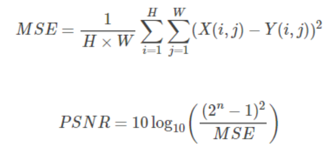
among ,n Is the number of bits per pixel .
PSNR Its unit is dB, The larger the value, the smaller the distortion , It is generally believed PSNR stay 38 The above time , The human eye cannot distinguish two pictures .
Related codes :
def psnr(loss): return 10 * log10(1 / loss.item())5.2 SSIM
SSIM(Structural Similarity) For structural similarity , It consists of three comparison modules : brightness 、 Contrast 、 structure .
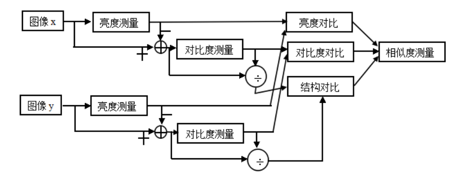
Brightness contrast function
Calculation formula of average gray level of image :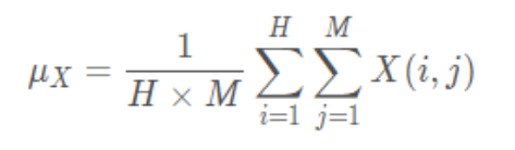
Calculation formula of brightness contrast function :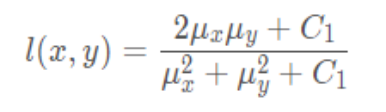
Contrast contrast function
Calculation formula of standard deviation of image :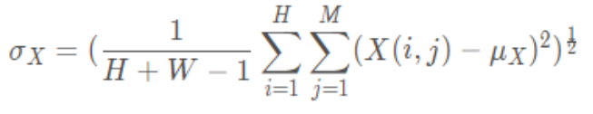
Calculation formula of contrast function :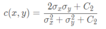
Structure comparison function
Structural comparison function calculation formula :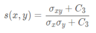
Combine the above three parts , obtain SSIM Calculation formula :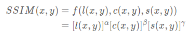
among ,,, > 0, To adjust the importance of these three modules .
SSIM The value range of the function is [0, 1], The larger the value, the smaller the image distortion , The more similar the two images are .
Related codes :
because pytorch There's nothing like tensorflow similar tf.image.ssim Calculate like this SSIM The interface of , Therefore, the user-defined function is used to calculate
""" Calculation ssim function """# Calculate one-dimensional Gaussian distribution vector def gaussian(window_size, sigma): gauss = torch.Tensor( [exp(-(x - window_size//2)**2/float(2*sigma**2)) for x in range(window_size)]) return gauss/gauss.sum()# Create Gaussian kernel , By matrix multiplication of two one-dimensional Gaussian distribution vectors # You can set channel The parameter is expanded to 3 passageway def create_window(window_size, channel=1): _1D_window = gaussian(window_size, 1.5).unsqueeze(1) _2D_window = _1D_window.mm( _1D_window.t()).float().unsqueeze(0).unsqueeze(0) window = _2D_window.expand( channel, 1, window_size, window_size).contiguous() return window# Calculation SSIM# Use it directly SSIM Formula , But when calculating the mean , Instead of directly averaging pixels , Instead, normalized Gaussian kernel convolution is used to replace .# Formulas are used in calculating variance and covariance Var(X)=E[X^2]-E[X]^2, cov(X,Y)=E[XY]-E[X]E[Y].def ssim(img1, img2, window_size=11, window=None, size_average=True, full=False, val_range=None): # Value range can be different from 255. Other common ranges are 1 (sigmoid) and 2 (tanh). if val_range is None: if torch.max(img1) > 128: max_val = 255 else: max_val = 1 if torch.min(img1) < -0.5: min_val = -1 else: min_val = 0 L = max_val - min_val else: L = val_range padd = 0 (_, channel, height, width) = img1.size() if window is None: real_size = min(window_size, height, width) window = create_window(real_size, channel=channel).to(img1.device) mu1 = F.conv2d(img1, window, padding=padd, groups=channel) mu2 = F.conv2d(img2, window, padding=padd, groups=channel) mu1_sq = mu1.pow(2) mu2_sq = mu2.pow(2) mu1_mu2 = mu1 * mu2 sigma1_sq = F.conv2d(img1 * img1, window, padding=padd, groups=channel) - mu1_sq sigma2_sq = F.conv2d(img2 * img2, window, padding=padd, groups=channel) - mu2_sq sigma12 = F.conv2d(img1 * img2, window, padding=padd, groups=channel) - mu1_mu2 C1 = (0.01 * L) ** 2 C2 = (0.03 * L) ** 2 v1 = 2.0 * sigma12 + C2 v2 = sigma1_sq + sigma2_sq + C2 cs = torch.mean(v1 / v2) # contrast sensitivity ssim_map = ((2 * mu1_mu2 + C1) * v1) / ((mu1_sq + mu2_sq + C1) * v2) if size_average: ret = ssim_map.mean() else: ret = ssim_map.mean(1).mean(1).mean(1) if full: return ret, cs return retclass SSIM(torch.nn.Module): def __init__(self, window_size=11, size_average=True, val_range=None): super(SSIM, self).__init__() self.window_size = window_size self.size_average = size_average self.val_range = val_range # Assume 1 channel for SSIM self.channel = 1 self.window = create_window(window_size) def forward(self, img1, img2): (_, channel, _, _) = img1.size() if channel == self.channel and self.window.dtype == img1.dtype: window = self.window else: window = create_window(self.window_size, channel).to( img1.device).type(img1.dtype) self.window = window self.channel = channel return ssim(img1, img2, window=window, window_size=self.window_size, size_average=self.size_average)6. model training / test
Set up epoch by 500 Time , Save on the validation set PSNR Highest model . The performance of the two models on the test set is shown in the following table :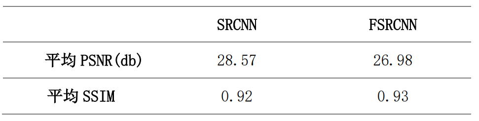
It can be found from the results that ,FSRCNN Of PSNR Than SRCNN low , but FSRCNN Of SSIM Than SRCNN high , explain PSNR and SSIM There is no completely positive correlation .
Training / Verification code :
model = FSRCNN(1).to(device)criterion = nn.MSELoss()optimizer = optim.Adam(model.parameters(), lr=1e-2)scheduler = MultiStepLR(optimizer, milestones=[50, 75, 100], gamma=0.1)best_psnr = 0.0for epoch in range(nb_epochs): # Train epoch_loss = 0 for iteration, batch in enumerate(trainloader): input, target = batch[0].to(device), batch[1].to(device) optimizer.zero_grad() out = model(input) loss = criterion(out, target) loss.backward() optimizer.step() epoch_loss += loss.item() print(f"Epoch {epoch}. Training loss: {epoch_loss / len(trainloader)}") # Val sum_psnr = 0.0 sum_ssim = 0.0 with torch.no_grad(): for batch in valloader: input, target = batch[0].to(device), batch[1].to(device) out = model(input) loss = criterion(out, target) pr = psnr(loss) sm = ssim(input, out) sum_psnr += pr sum_ssim += sm print(f"Average PSNR: {sum_psnr / len(valloader)} dB.") print(f"Average SSIM: {sum_ssim / len(valloader)} ") avg_psnr = sum_psnr / len(valloader) if avg_psnr >= best_psnr: best_psnr = avg_psnr torch.save(model, r"best_model_FSRCNN.pth") scheduler.step()Test code :
BATCH_SIZE = 4model_path = "best_model_FSRCNN.pth"testset = DatasetFromFolder(r"./data/images/test", zoom_factor)testloader = DataLoader(dataset=testset, batch_size=BATCH_SIZE, shuffle=False, num_workers=NUM_WORKERS)sum_psnr = 0.0sum_ssim = 0.0model = torch.load(model_path).to(device)criterion = nn.MSELoss()with torch.no_grad(): for batch in testloader: input, target = batch[0].to(device), batch[1].to(device) out = model(input) loss = criterion(out, target) pr = psnr(loss) sm = ssim(input, out) sum_psnr += pr sum_ssim += smprint(f"Test Average PSNR: {sum_psnr / len(testloader)} dB")print(f"Test Average SSIM: {sum_ssim / len(testloader)} ")7. Real map test
In order to intuitively feel the effect of the two models , I use my own pictures to test the real pictures , The effect is as follows :
s=1( Magnification =1)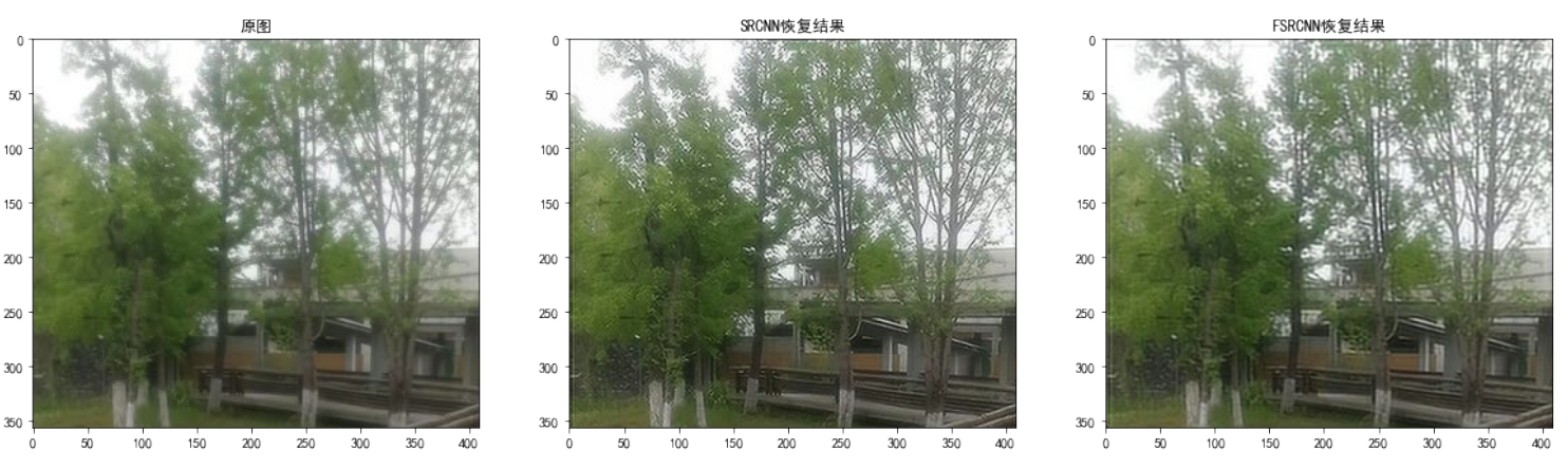
When the magnification =1 when ,SRCNN The super score result ratio of FSRCNN The super score effect of is better , This is on average with the two models PSNR The values of are consistent .
s=2( Magnification =2)

When the magnification =2 when ,SRCNN And FSRCNN There is little difference in the super score effect of .
Related codes :
# Parameter setting zoom_factor = 1model = "best_model_SRCNN.pth"model2 = "best_model_FSRCNN.pth"image = "tree.png"cuda = 'store_true'device = torch.device("cuda:0" if torch.cuda.is_available() else "cpu")# Read the picture img = Image.open(image).convert('YCbCr')img = img.resize((int(img.size[0] * zoom_factor), int(img.size[1] * zoom_factor)), Image.BICUBIC)y, cb, cr = img.split()img_to_tensor = transforms.ToTensor()input = img_to_tensor(y).view(1, -1, y.size[1], y.size[0]).to(device)# Output pictures model = torch.load(model).to(device)out = model(input).cpu()out_img_y = out[0].detach().numpy()out_img_y *= 255.0out_img_y = out_img_y.clip(0, 255)out_img_y = Image.fromarray(np.uint8(out_img_y[0]), mode='L')out_img = Image.merge('YCbCr', [out_img_y, cb, cr]).convert('RGB')model2 = torch.load(model2).to(device)out2 = model2(input).cpu()out_img_y2 = out2[0].detach().numpy()out_img_y2 *= 255.0out_img_y2 = out_img_y2.clip(0, 255)out_img_y2 = Image.fromarray(np.uint8(out_img_y2[0]), mode='L')out_img2 = Image.merge('YCbCr', [out_img_y2, cb, cr]).convert('RGB')# Drawing display fig, ax = plt.subplots(1, 3, figsize=(20, 20))ax[0].imshow(img)ax[0].set_title(" Original picture ")ax[1].imshow(out_img)ax[1].set_title("SRCNN Recovery results ")ax[2].imshow(out_img2)ax[2].set_title("FSRCNN Recovery results ")plt.show()fig.savefig(r"tree2.png")The source code for
Experimental report , Complete source code file , Data set acquisition :
https://download.csdn.net/download/qq1198768105/85906814
边栏推荐
- July Huaqing learning-1
- Select drop-down box realizes three-level linkage of provinces and cities in China
- 【无标题】
- mmclassification 训练自定义数据
- 【pytorch 修改预训练模型:实测加载预训练模型与模型随机初始化差别不大】
- The survey shows that traditional data security tools cannot resist blackmail software attacks in 60% of cases
- byte2String、string2Byte
- Matlab boundarymask function (find the boundary of the divided area)
- liunx禁ping 详解traceroute的不同用法
- 【Win11 多用户同时登录远程桌面配置方法】
猜你喜欢

Riddle 1

全网最全的新型数据库、多维表格平台盘点 Notion、FlowUs、Airtable、SeaTable、维格表 Vika、飞书多维表格、黑帕云、织信 Informat、语雀
![[loss functions of L1, L2 and smooth L1]](/img/c6/27eab1175766b77d4f030b691670c0.png)
[loss functions of L1, L2 and smooth L1]
The survey shows that traditional data security tools cannot resist blackmail software attacks in 60% of cases
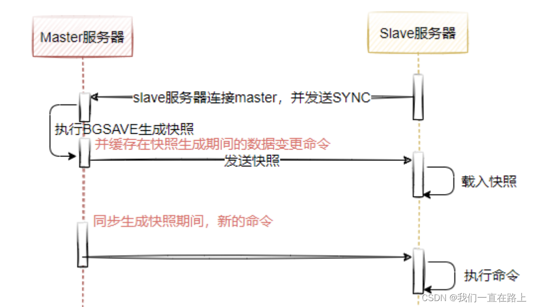
redis主从模式
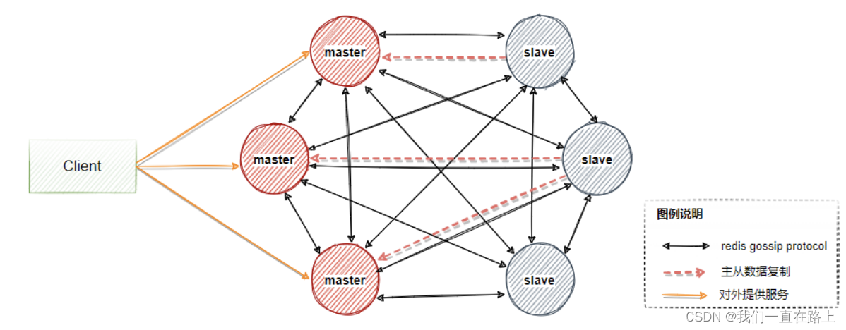
Principle of redis cluster mode
![[cloud native | kubernetes] actual battle of ingress case (13)](/img/1a/9404f6dcedd15827fa45f8f6f4c093.png)
[cloud native | kubernetes] actual battle of ingress case (13)
![[pytorch pre training model modification, addition and deletion of specific layers]](/img/cb/aa0b1116ec9b98e3ee5725aa58f4fe.png)
[pytorch pre training model modification, addition and deletion of specific layers]
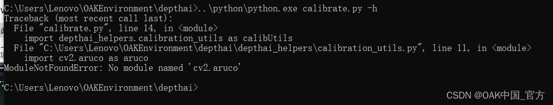
Error modulenotfounderror: no module named 'cv2 aruco‘
The most comprehensive new database in the whole network, multidimensional table platform inventory note, flowus, airtable, seatable, Vig table Vika, flying Book Multidimensional table, heipayun, Zhix

随机推荐
The solution of outputting 64 bits from printf format%lld of cross platform (32bit and 64bit)
【ijkplayer】when i compile file “compile-ffmpeg.sh“ ,it show error “No such file or directory“.
Want to ask, how to choose a securities firm? Is it safe to open an account online?
How to make your products as expensive as possible
Programmers are involved and maintain industry competitiveness
[singleshotmultiboxdetector (SSD, single step multi frame target detection)]
手机 CPU 架构类型了解
pytorch-线性回归
Which domestic cloud management platform manufacturer is good in 2022? Why?
JS for循环 循环次数异常
Course design of compilation principle --- formula calculator (a simple calculator with interface developed based on QT)
强化学习-学习笔记3 | 策略学习
【L1、L2、smooth L1三类损失函数】
16 channel water lamp experiment based on Proteus (assembly language)
Multi table operation - sub query
MVVM framework part I lifecycle
[pytorch modifies the pre training model: there is little difference between the measured loading pre training model and the random initialization of the model]
Redis master-slave mode
Reinforcement learning - learning notes 3 | strategic learning
[untitled]