当前位置：网站首页>Using tail as time series to identify whales

Using tail as time series to identify whales

2020-11-09 23:48:00 【Artificial intelligence meets pioneer】

author |Lamothe Thibaud
compile |Flin
source |towardsdatascience

Using curvature integral and dynamic time warping , Let's delve into sperm whale recognition ！

Preface

lately , We tried Capgemini Global data science challenge . I and Acores The whale research center works with , The challenge is to identify sperm whales , Using artificial intelligence to help save the lives of sperm whales .

In order to accomplish this task , We've collected thousands of pictures of whales from the past few years . In the training dataset , The average whale has 1.77 A picture , Many animals only appear once . therefore , The main idea is , Give a new picture , Find the closest to it from the existing data .

therefore , If the whale has been photographed , The researchers will be able to know when and where it was taken .

I am proud to announce , We finished the game with third place , We use Siam network It's a victory . however , Because there have been a lot of articles on this wonderful Architecture , Today I'm going to introduce a more interesting 、 A more novel way to solve this problem .

Method

from Weideman And so on , In their paper “ Curvature integral representation and matching algorithm for dolphin and whale recognition ” in , This is the key step of the method that I'm going to introduce today ：

Tail extraction based on color analysis and contour detection
Curvature integral tail treatment （IC）
And dynamic time warping （DTW） Compare the tail of

disclaimer N°1： The prediction rate is not as good as Siam network , We have to explore other solutions . But the idea is very interesting , It's worth sharing and understanding .

disclaimer N°2： In many data science projects , Data preparation is the most difficult part . actually , To process the tail as a signal , The quality of the signal has to be very good . In this paper , We will take some time to understand all the necessary steps before signal processing .

Explore our dataset , Analyze the pictures

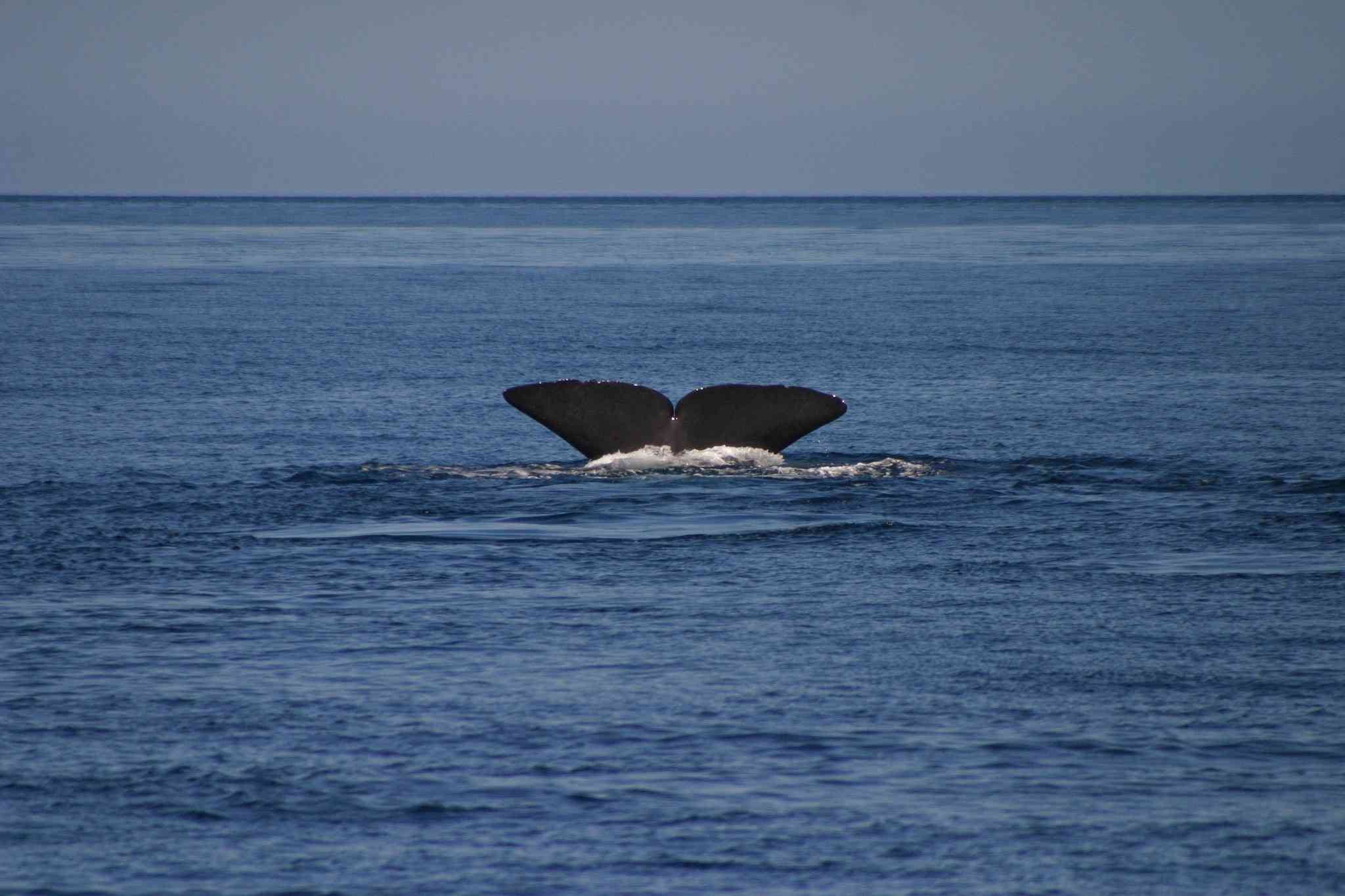
As stated in the introduction , We got thousands of pictures . At first glance , A whale is a whale . All of these pictures look like a blue background （ The sky and the sea ）, There's a gray spot in the middle （ tail ）.

After initial exploration , We started to distinguish between two different sperm whales , This is mainly due to the shape of the tail , We are convinced that this is crucial to our algorithm . What about the color ？ Is there any interesting information in the pixel distribution ？

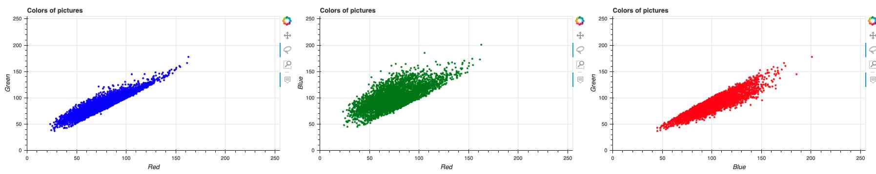
The correlation between the number of colors in each image （ Green and red – Blue and red – Green and blue ）
Use Bokeh Visualization Library （https://bokeh.org/） , We quickly found that the colors in the image are highly correlated . therefore , We focus on the contours , Try to detect them by color change .

Tail extraction based on color filter

The first step in detecting the profile of the tail is to extract the tail from the sky and water . actually , This is the most difficult part of the process .

First , We use contour detection Algorithm . But because the sun is constantly changing from one lens to another , So the contrast has changed a lot , The results are always unsatisfactory .

By the way , It's interesting to see where image algorithms fail most , Because in most cases , The difference between the tail and the sea is obvious to humans .

That being the case , Let's delve into color analysis and contour extraction Automation .

Use color to extract the tail

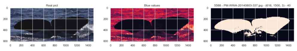
Let's give each channel strength （ Red , green , Blue ） Draw a grayscale picture

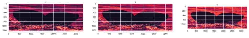
Look at the three channels of a single image

As you can see above , This is true for most pictures , Less color in the middle , You can filter by pixel strength . Because the tail is usually gray , So they have almost the same number of each color （R = G = B）, however , The sea and the sky are often blue , This makes the color ideal for filtering .

Let's see when only the blue value is retained , And only keep the blue value < Selected threshold （blue_value < SELECTED_THRESHOLD） What happens when the pixels are .

Selected threshold SELECTED_THRESHOLD The maximum value of is 255, Because it's the maximum pixel strength .

Through this series of pictures , We can believe that , It's easy to extract the tail . But how do I choose the filtering threshold ？

Here are the USES 10 To 170（ Ten times ten ） As a result example of the threshold value of a single picture .

According to the intensity of the blue pixels , Apply... To an image 17 Different filters ：

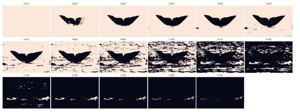
Here are some interesting things ：

The threshold is very small （ about 10）, The sea is gone , But the tail also disappeared
The threshold is very small （ about 20）, Part of the tail disappeared
The threshold is not too high （ about 40）, It's very well extracted , All the tails are not as blue as the threshold , But all the seas are bluer than the threshold .
At the intermediate threshold （ about 80） Under the circumstances , The tail remains intact , But we can only keep part of the ocean at first
At a threshold close to the median （ about 110） Under the circumstances , It's hard to tell the sea from the tail
At higher thresholds （>=140） Next , The tail completely disappeared . Even if the sea is blue enough , Cannot select through filter .

So here we are , And it seems obvious that SELECTED_THRESHOLD = 40 And Application filter blue_value < 40.

You can guess. , It's not easy . Given the light intensity of the image , The correct value for this image is 40. But it's a cliche too . By plotting all of these thresholds on random images , The threshold occurs at 10 To 130 Change between . So how to choose the right value ？

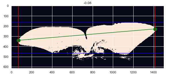
Use the bounding box to select the threshold

By looking at the front picture , We thought of something ： The correct image with the correct threshold is the image with the largest white space on the outside and the largest area on the inside . And hope some of them are in ImageNet The trained neural network can locate the whale in the picture . We decided to use the ImageNet Class MobileNet.

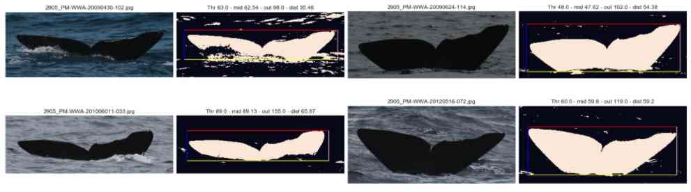
Compared with the original picture , A batch of extracted tails with borders

That's a good idea . As shown below , We can position the tail very accurately in the picture . then , We can put “ The tail - Inside ” And “ The sea - external ” Separate .

To better understand this separation , For each picture of the training set , We add the blue values of each pixel in the bounding box , And do the same for the pixels outside the frame .

then , Let's draw each picture on the diagram below , The internal results are reflected in X On the shaft , The external results are reflected in Y On the shaft . The blue line stands for X = Y. The meaning we can get from this graph is as follows ： The further away you are offline , The easier the separation between the tail and the ocean .

Compare sperm whale images with blue pixel intensities inside and outside the bounding box

We try to apply filter thresholds based on the distance from the line , But it didn't produce any results . After several attempts , We can't do anything based on the color distribution of the picture , So decided to take a tough approach . In addition to looking at pictures and determining thresholds , We also apply 15 A filter , Analyze it , Then the best filter is automatically selected for further processing .

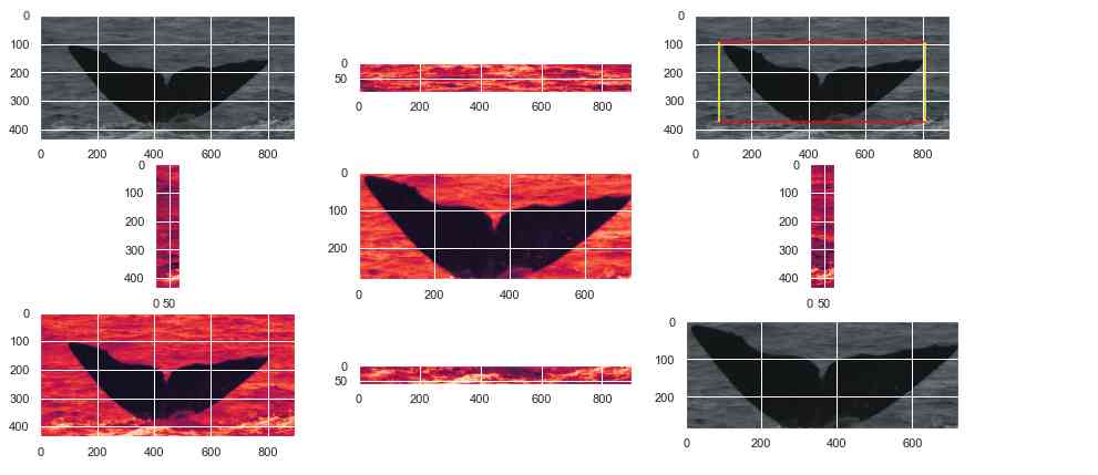
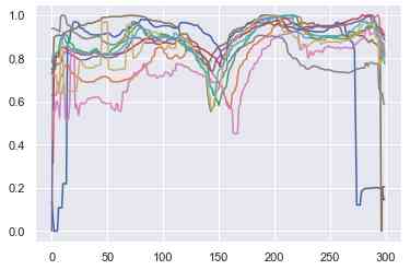
And then for a given picture , We will 15 Filters have been applied 15 Different values as thresholds . For each filter , We calculate the number of pixels inside and outside the bounding box （ After filtration , The pixel value is 0 or 1, There's no need to sum the strengths ）. then , We normalize the results , Make the number independent of the size of the image , And draw the results on a graph .

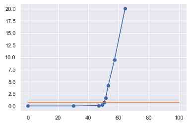
Single image and different filtering thresholds within the bounding box （X Axis ） And the outer frame （Y Axis ） The number of pixels .

For each picture , We get curves that are similar to the curves above , This is our mathematical transformation of the previous statement as the threshold evolves .

When the threshold is small , The tail and the sea are gone . There are no pixels inside or outside the tail
When the threshold increases , There's a tail , also X The value of the axis increases .
Until the threshold starts to appear in some parts of the ocean , And external value began to grow .

Use linear regression or derivative , Now it's easy to detect the right threshold ： It is the threshold at the intersection of two lines of a graph .

Be careful ： The orange line is y = y_of_the_selected_threshold

The last hint of tail extraction

Last , In order to get the best picture when extracting , When we figure out the best threshold （10,20,30,40,…,120,130,140,150） when , The assumption is 80. We are right. -5/+5 Value applies a filter . So we have three pictures ： Blue < 75, Blue < 80, Blue < 85. Then we take three of these grid images （0 and 1） Sum up , And only keep the value of the resulting pixel equal to 2. This will serve as the final filter , Remove the noise from the tail . This kind of extraction effect is very good , We decided to apply it to all the pictures .

result

As a summary , Here are the assumptions we've made so far ：

We can use the intensity of the blue pixels to distinguish the tail from the ocean
Before filtering , You need to find a threshold for each image
Using a bounding box is an effective way to find this threshold

After hours of work , We ended up with a very good tail extractor , It works well with different brightness , The weather , Ocean color , Tail color tail , And be able to view the most difficult pictures .

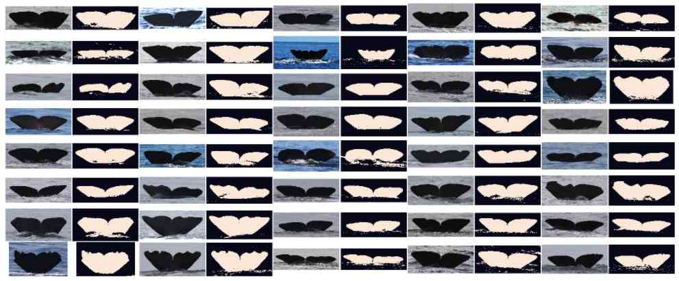
A batch of extracted tails are compared with the original image

Contour detection

Now the tail is in the picture , We do contour detection . exactly , To deal with tails in time series , We need to signal .

In this step , We can use OpenCV The contour detection algorithm of , But through the following two steps , It's going to look faster ：

step 1： Use entropy to remove noise around the tail

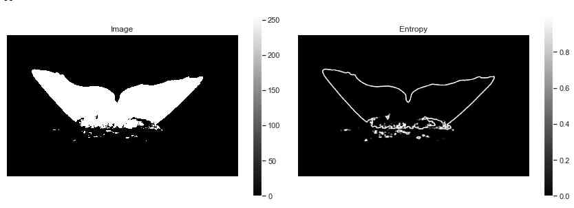
Use entropy change to keep only the outline of the extracted tail

step 2： Keep the highlight pixels of each column of pictures

The extracted tail contour detected after applying the entropy filter

This step is very simple , There's no complexity .

Curvature integral

By extracting the tail from the sea and getting the upper pixel of the image , We got the back edge of the tail as a signal . Now we have this , We have to deal with standardization . actually , All pictures are different in size or number of pixels . Besides , The distance to the sperm whale is not always the same , The orientation may change when shooting .

An example of tail orientation , There may be differences between two pictures of the same whale

For Standardization , We have to go along two axes . First , We decided to use each tail 300 Point to point comparison . Then we interpolate the shortest interpolation , And sample the longest one . secondly , We will 0 To 1 Normalization of all values between . This causes the signal to stack up , As shown in the figure below .

Scale signal superposition

To solve the problem of orientation , We use the curvature integral measure , This metric converts a signal into another signal by local evaluation .

As stated in the original paper ：“ It captures the local shape information of each point along the trailing edge . For a given point on the trailing edge , We place a radius at this point r The circle of , Then find all the points on the trailing edge that lie within the circle .”

then , At each step , Pull our signal straight along the edge of the circle , So that it is inscribed as a square .

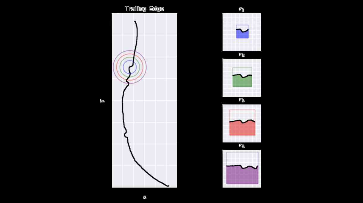
Curvature integral principle

Last , We define curvature as follows ：

Curvature is the area under the curve to the total area of the square , This means that the curvature of the line is c = 0.5

therefore , We've got standardized signals , It's not about the distance between the whale and the photographer , It's not about the angle between the whale and the photographer , And it's not about the angle between the whale and the ocean .

then , For each training test picture , We are IC During the phase shift, the radii are created 5、10 and 15 Those signals in pixels . We store them , And for the last step ： Comparison between time series .

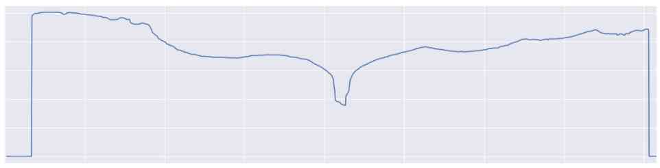
In this paper , I will introduce the implementation of this algorithm . Once working , We can apply it to the trailing edge , And extract signals from environmental details . For a tail , The signal looks like this ：

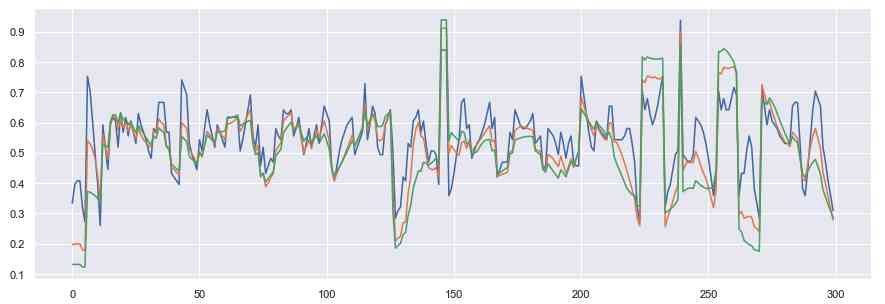
The curvature integral is applied to the case with 3 The tail edge of sperm whale with different radius values

Now? , Let's compare the signals ！

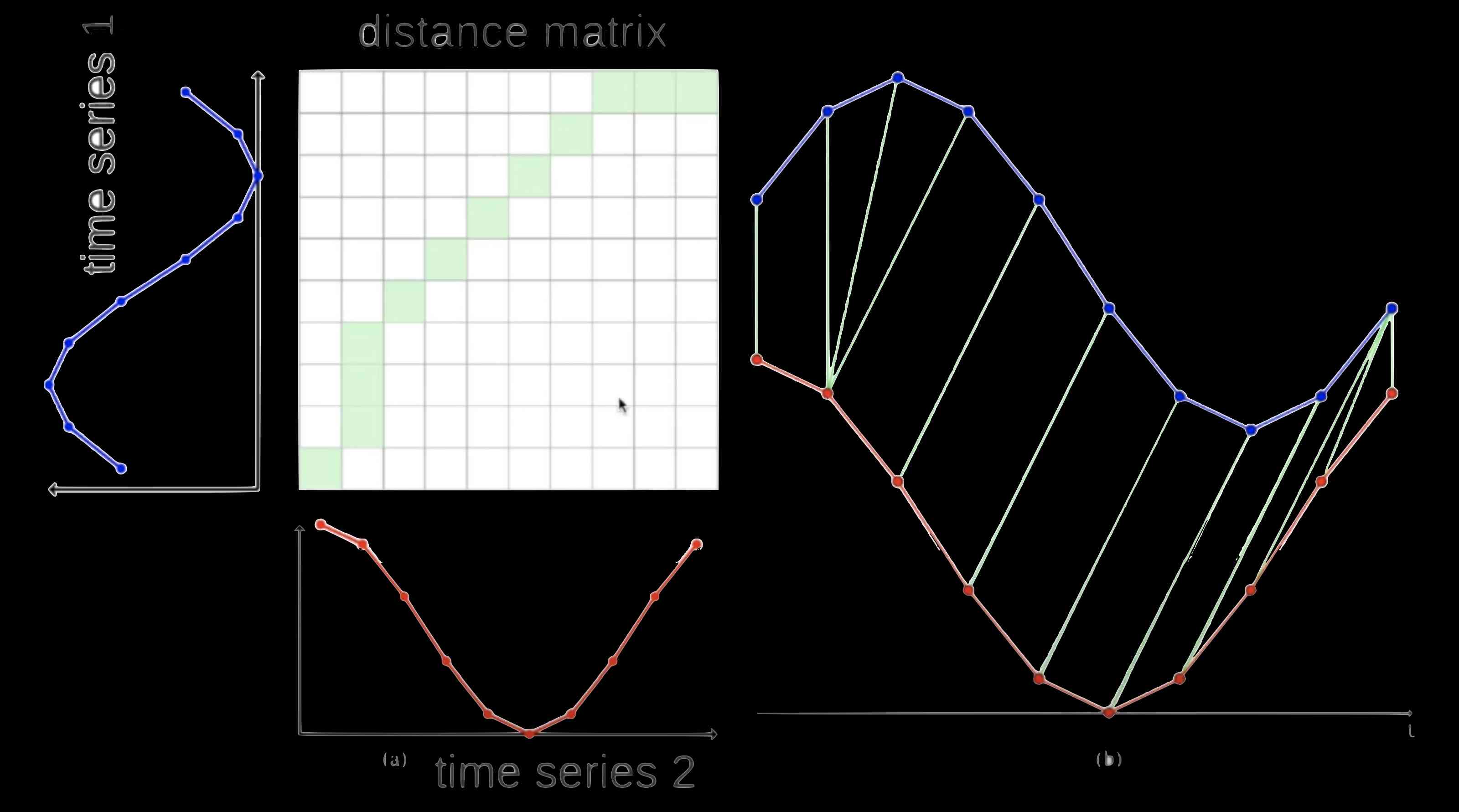
Dynamic time regulation

Dynamic time regulation （DTW,https://en.wikipedia.org/wiki/Dynamic_time_warping） It is an algorithm that can find the best alignment between two time series . It is usually used to determine the similarity of time series , Classify and find the corresponding area between two time series .

Distance from Euclid （ finger It's the distance between two curves , Point by point ） contrary ,DTW Distance allows different parts of the curve to be linked . The principle of the algorithm is as follows ：

Use 2 Curves , We created a distance matrix between two series , From the bottom left to the top right , Calculate the distance between two points Ai and Bi, Calculate the distance between the two points as follows ：D(Ai, Bi) = |Ai — Bi] + min(D[i-1, j-1], D[i-1, j], D[i, j-1]).

When the distance matrix satisfies , We calculate the path with less weight from the upper right corner to the lower left corner . So , We choose the square with the smallest value in each step .

Last , The chosen path （ The green in the picture below ） Indication from sequence A Which data point corresponds to the sequence B Data points in .

This kind of basic computing is very easy to implement . for example , This is one based on two sequences s And the function that creates the distance matrix t.

def dtw(s, t):
  """ Computes the distance matrix between two time series
      args: s and t are two numpy arrays of size (n, 1) and (m, 1)
  """
  
    # Instanciate distance matrix
    n, m = len(s), len(t)
    dtw_matrix = np.zeros((n+1, m+1))
    for i in range(n+1):
        for j in range(m+1):
            dtw_matrix[i, j] = np.inf
    dtw_matrix[0, 0] = 0
    
    # Compute distance matrix
    for i in range(1, n+1):
        for j in range(1, m+1):
            cost = abs(s[i-1] - t[j-1])
            last_min = np.min([
              dtw_matrix[i-1, j],
              dtw_matrix[i, j-1],
              dtw_matrix[i-1, j-1]
            ])
            dtw_matrix[i, j] = cost + last_min
    
    return dtw_matrix

That being the case , Let's go back to our sperm whales ！ Each tail of the dataset is converted to “ Integral curve signal ”, We calculated the distance between all the tails , To find the closest .

after , When a new picture is received , We have to get it through the whole preparation process ： Use the tail of the blue filter to extract , Using entropy method for contour detection and using IC Perform contour conversion . It gave us a 300x1 The tensor of shape , Finally, we need to calculate the distance of the entire dataset . By the way , It takes time .

Sentence ： The results are impressive ！ When we have two pictures of the same whale , in the majority of cases , The two photos are the closest 40 Zhang , This is in 2000 The middle of the year is the best . however , As stated in the introduction , The result of using Siam network is better than this photo （ Pictures are usually in the nearest 5 Zhang Zhong ））, Given the time of the game , We have to choose other methods in the investigation .

Reward ： Processing half the tail and half the signal

We try to use the half tail , Suppose any of the following ：

The tail is symmetrical , This will simplify the calculation .
The tail is asymmetrical , So you can compare it with the half tail .

Despite a lot of testing , But that doesn't give us very definite results . We don't think our separation is reliable enough ： We will need more time to study the better separation that signal processing brings .

The last thought

After sending some tail fetches that are harder than we thought , Because of the color of the picture （ It's basically blue —— The sea and the sky ） And the brightness of the images in the dataset , We use two continuous processing methods for tail recognition .

First , Curvature integral is a method of normalizing the signal by looking at the local changes of the curve . then , We use dynamic time warping , This is the distance between two curves , Even if you move two curves, you may find similarities between them .

Unfortunately , It didn't turn out to be what I wanted , We can't continue to use the solution . Through more time and more effort , I'm confident that we can improve every step of the pipeline , To get a better model . I also enjoy working with the concepts mentioned in this article .

Through all the steps , Different ways to implement them and parameters , Monitoring all transitions is very challenging . Just as we have a roadmap , Each step has its own difficulties , Every little success is a victory , It opens up the next step . Very gratifying .

I find this method very interesting , And with the usual pre training CNN Completely different . I hope you also like the advantages of this approach in this article . If you have any questions , Please feel free to contact me