Notes on the paper "cross view transformers for real time map view semantic segmentation"

Reference code ：cross_view_transformers

1. summary

Introduce ： This article proposes a new 2D Dimensional bev Feature extraction scheme , It introduces camera prior information （ Camera internal and external parameters ） Build a multi view cross attention mechanism , It can map multi view features to BEV features . For building its multi view feature bev Bridge of feature mapping relationship , This is through BEV Location code （ You need to add the original bev queries As refine, For what is written here “ code ” That is, in the text embedding） And according to the camera calibration results （ Internal and external parameters ） The camera position code obtained by calculation （camera-aware embedding）、 Multi view features do attention obtain , This step is called cross view attention. On the whole, the network front-end of the article is used CNN As a feature extraction network , Middle end use CNN Multi level features are optimized in multi view as input BEV features （ That is, cascade optimization is used ）, The back-end using CNN Form decoder for output . The overall operation is simple and efficient , In the 2080Ti GPU Achieve real-time effect on .

This article proposes based on transformer Of bev Feature extraction network （ about 2D Of bev）, about bev Under the queries By adding map-view embedding Conduct refine Get the final queries. Also in multi view features （ from CNN Network get ） Will also add camera-view Of embedding Conduct refine obtain key. At the same time, in order to feel the way 3D Positional geometry also determines the position of the camera embedding（ In the code, it is subtraction ）, And with the above two embedding Association . Finally, the original multi view feature will also be mapped as val, Build like this attention Calculation . The above mentioned contents can be seen in the following figure as an auxiliary explanation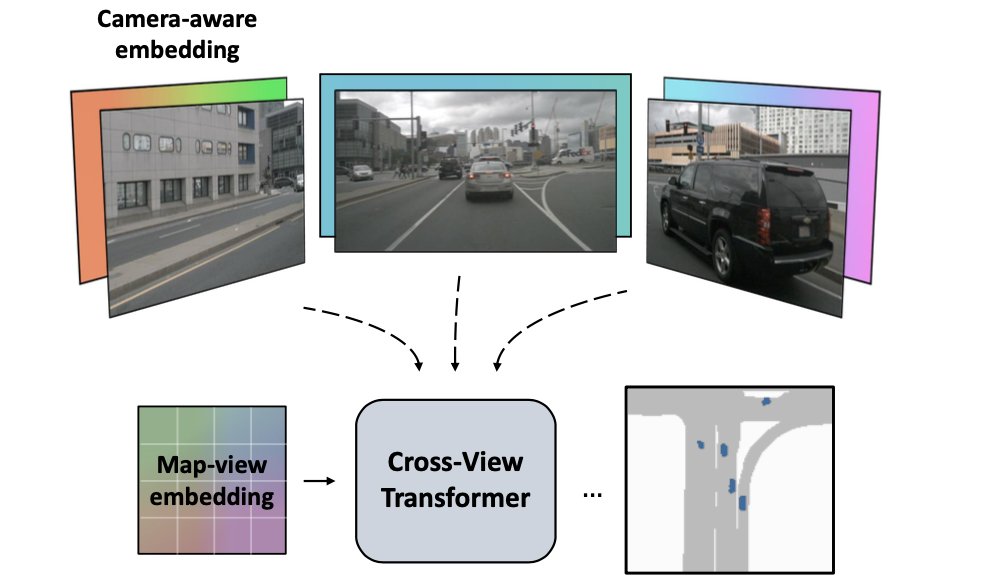

2. Methods to design

2.1 The Internet pipeline

The overall algorithm proposed in this paper is shown in the figure below ：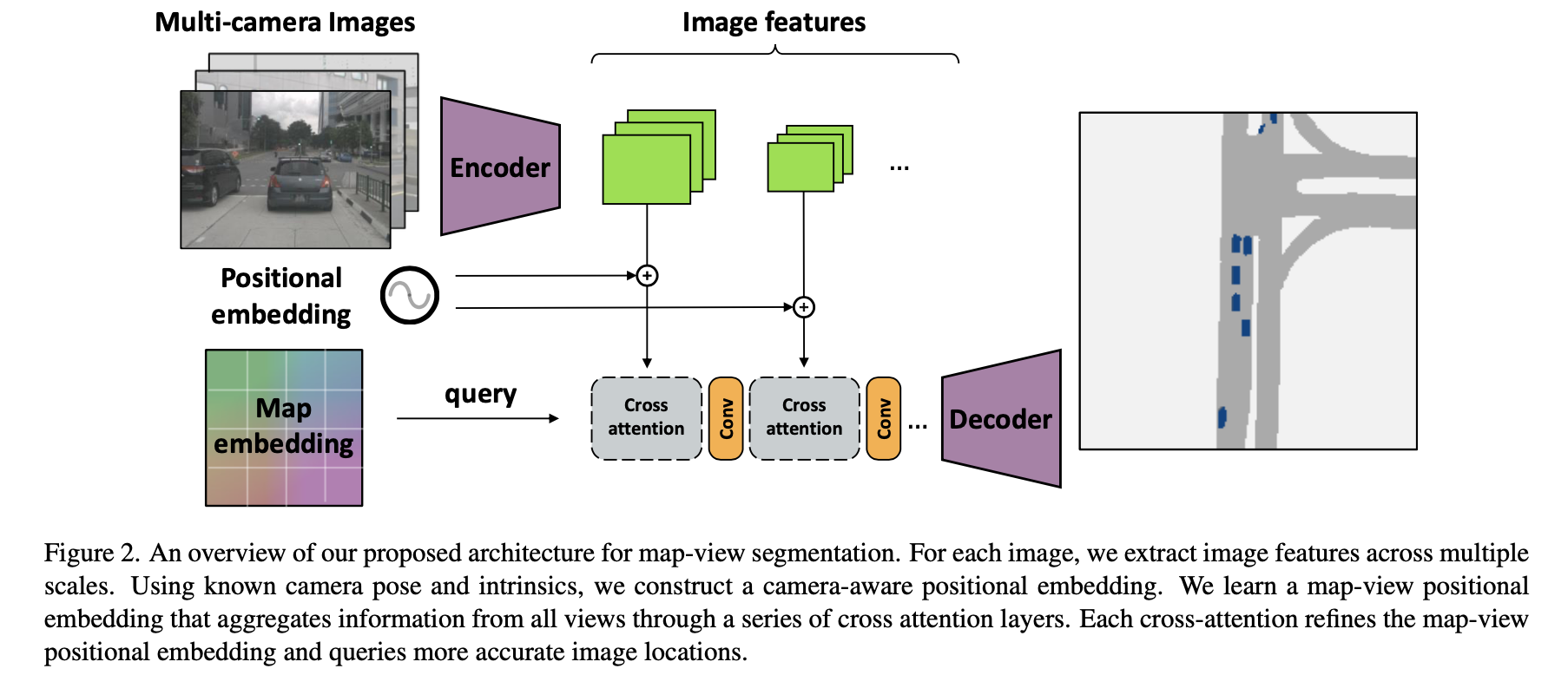

The data entered in the above figure is multi view data $\{I_k\in R^{W\ast H\ast 3},R_k\in R^{3\ast 3},K_k\in R^{3\ast 3},t_k\in R^3{\}}_{k=1}^n$（ Each represents the image 、 Rotation matrix 、 Internal parameter matrix 、 Translation vector ）. The final structure is obtained through the following steps ：

• 1）CNN The network extracts from multi view data CNN features ${\delta }_k,k=1,\dots ,n$, These features will be mapped by a linetype attention Medium val.
• 2）CNN Add camera-view embedding（ It's the one in the picture above positional embedding, It depends on the internal and external parameter matrix obtained by the calibration of their respective views ） As refine To get attention Medium key.
• 3）bev Of queries Will be in map embedding（bev grid adopt embedding And then get ） Next refine Get to the end attention Of queries.
• 4） Use CNN The multi-level characteristic graph output by the network adopts the cascade method refine bev features , Then it is sent to the decoding unit to get the output result .

2.2 cross view attention

stay 3D In this case, point space point $x^{(W)}$ And image points $x^{(I)}$ The mapping relationship of is ：
$$x^{(I)}\simeq K_k{R}_k(x^{(W)}-t_k)$$
That is to say, the above situation is only approximately equal , The actual depth value is unknown , Desire exists scale The uncertainty on . In this article, we do not explicitly use depth information or implicitly encode the spatial distribution of depth , It's going to be scale The uncertainty code on uses the above mentioned camera-view embedding、map-view embedding and transformer Network for learning and adaptation . As for the above mentioned 3D Space point $x^{(W)}$ And image points $x^{(I)}$ The similarity relation of uses cosine similarity ：
$$si{m}_k(x^I,x^{(W)})=\frac{(R_k^{-1}{K}_k^{-1}{x}^{(I)})\cdot (x^W-t_k)}{||R_k^{-1}{K}_k^{-1}{x}^{(I)}||||x^W-t_k||}$$

camera-view embedding:
Here, the position coding is carried out in the feature dimension of multiple views in combination with the camera internal and external parameters of each view , That is, map each pixel on the feature map to 3D Space goes ：
$$d_{k,i}=R_k^{-1}{K}_k^{-1}{x}_i^{(I)}$$
After mapping 3D Points will be encoded through a linear network camera-view embedding（${\delta }_{k,i}\in R^D$）, Refer to the following code ：

# cross_view_transformer/model/encoder.py#L248
pixel_flat = rearrange(pixel, '... h w -> ... (h w)')                   # 1 1 3 (h w)
cam = I_inv @ pixel_flat                                                # b n 3 (h w)
cam = F.pad(cam, (0, 0, 0, 1, 0, 0, 0, 0), value=1)                     # b n 4 (h w)
d = E_inv @ cam                                                         # b n 4 (h w)
d_flat = rearrange(d, 'b n d (h w) -> (b n) d h w', h=h, w=w)           # (b n) 4 h w
d_embed = self.img_embed(d_flat)                                        # (b n) d h w

...

if self.feature_proj is not None:  # linear projection refine
    key_flat = img_embed + self.feature_proj(feature_flat)              # (b n) d h w
else:
    key_flat = img_embed                                                # (b n) d h w

Further, this code will subtract the camera position code ${\tau }_k\in R^D$（ The calculation process is the same as the above camera-view embedding The calculation process is similar to ）, The purpose is to estimate the 3D Space location . be camera-view embedding The influence of different calculation processes on performance is shown in the following table ：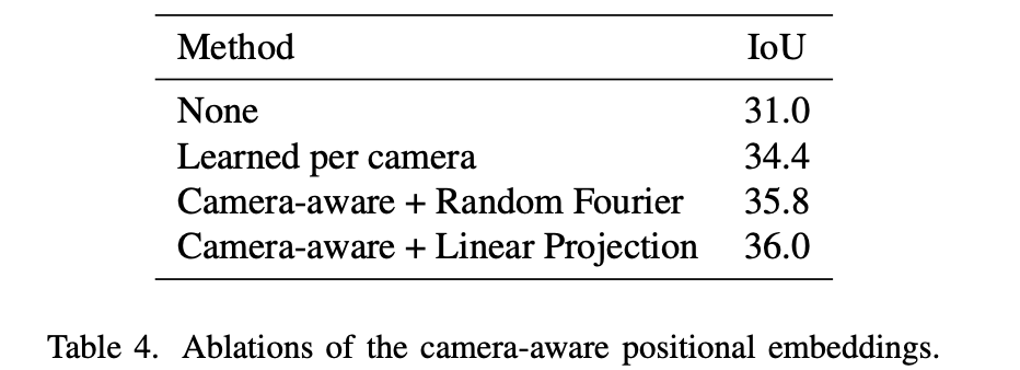

map-view embedding：
This part is in bev grid embedding Based on position coding with camera ${\tau }_k\in R^D$ What you can do badly （ Write it down as $c_j^n$）, It is different from the original bev queries Together into transformer Finish in attention, Its implementation can refer to ：

# cross_view_transformer/model/encoder.py#L258
world = bev.grid[:2]                                                    # 2 H W
w_embed = self.bev_embed(world[None])                                   # 1 d H W
bev_embed = w_embed - c_embed                                           # (b n) d H W
bev_embed = bev_embed / (bev_embed.norm(dim=1, keepdim=True) + 1e-7)    # (b n) d H W
query_pos = rearrange(bev_embed, '(b n) ... -> b n ...', b=b, n=n)      # b n d H W

feature_flat = rearrange(feature, 'b n ... -> (b n) ...')               # (b n) d h w

...

# Expand + refine the BEV embedding
query = query_pos + x[:, None]                                          # b n d H W

cross-view attention：
The mapped multi view features ${\varphi }_{k,i}$（ As val） With the above queries and key Conduct attention operation , For the article, the cosine similarity of the following form is used ：
$$sim({\delta }_{k,i},{\varphi }_{k,i},c_j^{(n)},{\tau }_k)=\frac{({\delta }_{k,i}+{\varphi }_{k,i})\cdot (c_j^n-{\tau }_k)}{||{\delta }_{k,i}+{\varphi }_{k,i}||||c_j^n-{\tau }_k||}$$

The impact of the above mentioned variables on performance ：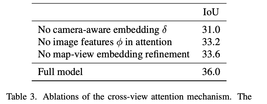

3. experimental result

nuScenes and Argoverse Data recording bev Segmentation performance comparison ：

Different bev setting and FPS Compare ：