当前位置:网站首页>Time convolution Network + soft threshold + attention mechanism to realize residual life prediction of mechanical equipment
Time convolution Network + soft threshold + attention mechanism to realize residual life prediction of mechanical equipment
2022-07-07 22:30:00 【Eva215665】
1. About data
This model adopts PHM2012 The whole life data of bearings in the data competition , as well as XJUST-SY The public data set of bearing life cycle is verified . Both are public datasets , Can own Baidu /Bing/Google download , And learn how to organize data files . This example only takes PHM2012 Take the data ,XJUST-SY Data only needs to replace the data storage path , The code doesn't need to change .
2. The code is not explained in detail
2.1 Import necessary Libraries
from keras.layers import Input,concatenate,GRU,Embedding,UpSampling1D,BatchNormalization,Conv1D,MaxPooling1D,Dense,Flatten,Lambda,Dropout,Concatenate,LeakyReLU,BatchNormalization,Reshape,Activation,GlobalAveragePooling1D,AveragePooling1D
from keras import regularizers
from keras.callbacks import EarlyStopping
from keras.optimizers import Adam
from keras.models import Sequential, Model
from keras import backend as K
from keras import Model,regularizers

from scipy import signal
import tensorflow as tf
import numpy as np
import matplotlib.pyplot as plt
from sklearn.model_selection import train_test_split
from sklearn.metrics import mean_squared_error
import xlrd
import os
from sklearn.preprocessing import MinMaxScaler
from keras.models import load_model

import keras
config = tf.ConfigProto()
config.gpu_options.allow_growth = True
keras.backend.tensorflow_backend.set_session(tf.Session(config=config))

import os
os.environ['CUDA_VISIBLE_DEVICES'] = '/gpu:0'
2.2 Write function , Import data
PHM2010 data Full_Test_Set Under folder Bearing1_4 In the data , Adopted ; The separator will be 、 branch 、 second 、x Acceleration in the direction of 、y Write a... To all acceleration values excel Cells of , It is inconsistent with several other file formats , So I wrote two functions , For reading Bearing1_4 Data under and data under other folders .
Read non Bearing1_4 Functions of data
# Read the horizontal signal from the folder csv data
def readfile_h(path):
    files = os.listdir(path)
    # take acc Pick out the documents
    files = list(filter(lambda x: x[0:4]=='acc_' , files))
    # Solve the disorder problem , By the end of 5 Bit to last 4 Sort the size of numbers between bits
    files.sort(key=lambda x:int(x[5:-4]))

    rowdata = []
    for file in files:
        info = path+"/"+file
        # take csv The data in the file is converted into a matrix
        data = np.loadtxt(open(info,"rb"), delimiter=',', skiprows=0)
        rowdata = np.hstack((rowdata,data[:,5]))
    return(rowdata)
The following read is not Bearing1_4 data
## 2803 individual csv file
train1_1_h = readfile_h('xxxx\Learning_set\Bearing1_1')
#871 individual csv file
train1_2_h = readfile_h('xxxx\Learning_set\Bearing1_2')
test1_3_h = readfile_h('xxxx\Full_Test_Set\Bearing1_3')
test1_5_h = readfile_h('xxxx\Full_Test_Set\Bearing1_5')
test1_6_h = readfile_h('xxxx\Full_Test_Set\Bearing1_6')
test1_7_h = readfile_h('xxxx\Full_Test_Set\Bearing1_7')
The following is read Bearing1_4 Functions of data
# Read 1_4 The data of
def readfile_h(path):
    files = os.listdir(path)
    # take acc Pick out the documents
    files = list(filter(lambda x: x[0:4]=='acc_' , files))
    # Solve the disorder problem , By the end of 5 Bit to last 4 Sort the size of numbers between bits
    files.sort(key=lambda x:int(x[5:-4]))

    rowdata = []
    for file in files:
        info = path+"/"+file
        # take csv The data in the file is converted into a matrix
        data = np.loadtxt(open(info,"rb"), delimiter=';',skiprows=0)
        rowdata = np.hstack((rowdata,data[:,5]))
    return(rowdata)
Read below Bearing1_4 data
test1_4_h = readfile_h('xxxx\Full_Test_Set\Bearing1_4')
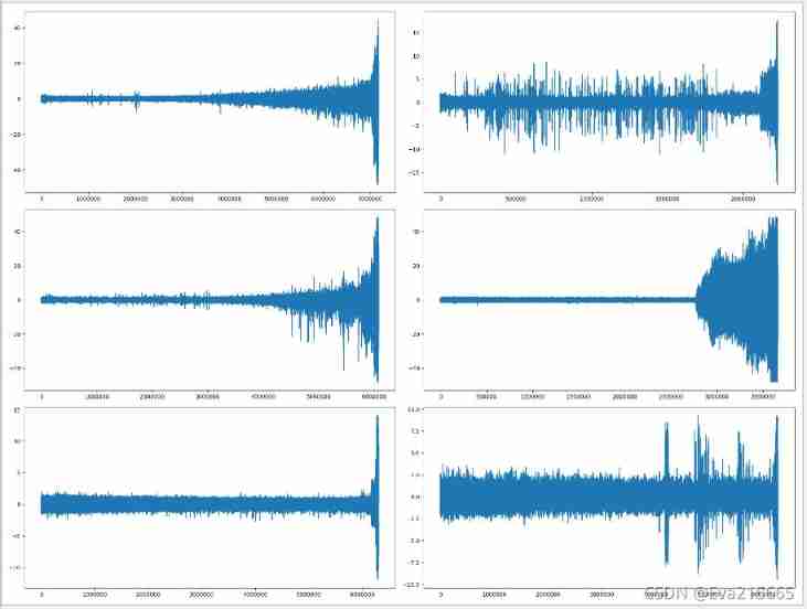
Print out the whole life data
plt.figure(figsize=(20,15))
plt.subplot(3, 2, 1)
plt.plot(train1_1_h)
plt.subplot(3, 2, 2)
plt.plot(train1_2_h)
plt.subplot(3, 2, 3)
plt.plot(test1_3_h)
plt.subplot(3, 2, 4)
plt.plot(test1_4_h)
plt.subplot(3, 2, 5)
plt.plot(test1_5_h)
plt.subplot(3, 2, 6)
plt.plot(test1_6_h)
plt.show()
The following is data standardization ,reshape Wait for pretreatment
#%%
# Standardize data
mean1_1 =train1_1_h - np.mean(train1_1_h)
train1_h = mean1_1/np.std(train1_1_h)

mean1_2 =train1_2_h - np.mean(train1_2_h)
train2_h =mean1_2/ np.std(train1_2_h)

mean1_3 =test1_3_h - np.mean(test1_3_h)
test3_h = mean1_3/np.std(test1_3_h)

mean1_5 =test1_5_h - np.mean(test1_5_h)
test5_h = mean1_5 /np.std(test1_5_h)

mean1_6 =test1_6_h - np.mean(test1_6_h)
test6_h = mean1_6 /np.std(test1_6_h)

mean1_7=test1_7_h - np.mean(test1_7_h)
test7_h = mean1_7 /np.std(test1_7_h)

mean1_4 =test1_4_h - np.mean(test1_4_h)
test4_h = mean1_4/np.std(test1_4_h)

xtr1_h=train1_h.reshape((-1,2560,1))
xtr2_h=train2_h.reshape((-1,2560,1))
xte3_h= test3_h.reshape(-1,2560,1)
xte4_h= test4_h.reshape(-1,2560,1)
xte5_h = test5_h.reshape(-1,2560,1)
xte6_h = test6_h.reshape(-1,2560,1)
xte7_h = test7_h.reshape(-1,2560,1)
print(xtr1_h.shape)
print(xtr2_h.shape)
print(xte3_h.shape)
print(xte4_h.shape)
print(xte5_h.shape)
print(xte6_h.shape)
print(xte7_h.shape)
The following is to write a function and read y Acceleration signal in direction , This can actually be compared with “ Read x Direction acceleration ” To optimize the function of
def readfile_v(path):
    files = os.listdir(path)
    # take acc Pick out the documents
    files = list(filter(lambda x: x[0:4]=='acc_' , files))
    # Solve the disorder problem , By the end of 5 Bit to last 4 Sort the size of numbers between bits
    files.sort(key=lambda x:int(x[5:-4]))

    rowdata = []
    for file in files:
        info = path+"/"+file
        # take csv The data in the file is converted into a matrix
        data = np.loadtxt(open(info,"rb"), delimiter=',',skiprows=0)
        rowdata = np.hstack((rowdata,data[:,4]))
    return(rowdata)

# Read working condition 1 The data of 、
# Training data
#2803 individual csv file
train1_1_v = readfile_v('xxxx\Learning_set\Bearing1_1')
#871 individual csv file
train1_2_v = readfile_v('xxxx\Learning_set\Bearing1_2')

# Test data
#test_data  Medium 2302 File
test1_3_v = readfile_v('xxxx\Full_Test_Set\Bearing1_3')
test1_5_v = readfile_v('xxxx\Full_Test_Set\Bearing1_5')
test1_6_v = readfile_v('xxxx\Full_Test_Set\Bearing1_6')
test1_7_v = readfile_v('xxxx\Full_Test_Set\Bearing1_7')

# Attempt to read 1_4 The data of
def readfile_v(path):
    files = os.listdir(path)
    # take acc Pick out the documents
    files = list(filter(lambda x: x[0:4]=='acc_' , files))
    # Solve the disorder problem , By the end of 5 Bit to last 4 Sort the size of numbers between bits
    files.sort(key=lambda x:int(x[5:-4]))

    rowdata = []
    for file in files:
        info = path+"/"+file
        # take csv The data in the file is converted into a matrix
        data = np.loadtxt(open(info,"rb"), delimiter=';',skiprows=0)
        rowdata = np.hstack((rowdata,data[:,4]))
    return(rowdata)

test1_4_v = readfile_v('xxxx\Full_Test_Set\Bearing1_4')
take y- Print out the directional acceleration signal
plt.figure(figsize=(20, 15))
plt.subplot(3, 2, 1)
plt.plot(train1_1_v)
plt.subplot(3, 2, 2)
plt.plot(train1_2_v)
plt.subplot(3, 2, 3)
plt.plot(test1_3_v)
plt.subplot(3, 2, 4)
plt.plot(test1_4_v)
plt.subplot(3, 2, 5)
plt.plot(test1_5_v)
plt.subplot(3, 2, 6)
plt.plot(test1_6_v)
plt.show()
The following is data standardization 、reshape Wait for pretreatment
# Standardize data
mean1_1 =train1_1_v - np.mean(train1_1_v)
train1_v = mean1_1/np.std(train1_1_v)

mean1_2 =train1_2_v - np.mean(train1_2_v)
train2_v =mean1_2/ np.std(train1_2_v)


mean1_3 =test1_3_v - np.mean(test1_3_v)
test3_v = mean1_3/np.std(test1_3_v)

mean1_4 =test1_4_v - np.mean(test1_4_v)
test4_v = mean1_4/np.std(test1_4_v)

mean1_5 =test1_5_v - np.mean(test1_5_v)
test5_v = mean1_5 /np.std(test1_5_v)


mean1_6 =test1_6_v - np.mean(test1_6_v)
test6_v = mean1_6 /np.std(test1_6_v)

mean1_7=test1_7_v - np.mean(test1_7_v)
test7_v = mean1_7 /np.std(test1_7_v)

xtr1_v = train1_v.reshape((-1, 2560, 1))
xtr2_v = train2_v.reshape((-1, 2560, 1))
xte3_v = test3_v.reshape((-1, 2560, 1))
xte4_v = test4_v.reshape((-1, 2560, 1))
xte5_v = test5_v.reshape((-1, 2560, 1))
xte6_v = test6_v.reshape((-1, 2560, 1))
xte7_v = test7_v.reshape((-1, 2560, 1))
print(xtr1_v.shape)
print(xtr2_v.shape)
print(xte3_v.shape)
print(xte4_v.shape)
print(xte5_v.shape)
print(xte6_v.shape)
print(xte7_v.shape)
Splice the horizontal signal and the vertical signal
# Splice the vertical signal and horizontal signal together
xtr1 = np.hstack((xtr1_v,xtr1_h))
xtr1 = xtr1.reshape((-1,2560,2))
xtr2 = np.hstack((xtr2_v,xtr2_h))
xtr2 = xtr2.reshape((-1,2560,2))
xte3 = np.hstack((xte3_v,xte3_h))
xte3 = xte3.reshape((-1,2560,2))
xte4 = np.hstack((xte4_v,xte4_h))
xte4 = xte4.reshape((-1,2560,2))
xte5 = np.hstack((xte5_v,xte5_h))
xte5 = xte5.reshape((-1,2560,2))
xte6 = np.hstack((xte6_v,xte6_h))
xte6 = xte6.reshape((-1,2560,2))
xte7 = np.hstack((xte7_v,xte7_h))
xte7= xte7.reshape((-1,2560,2))
print(xtr1.shape)
print(xtr2.shape)
print(xte3.shape)
print(xte4.shape)
print(xte5.shape)
print(xte6.shape)
print(xte7.shape)
Set up RUL Of ground truth
# Data labels , Remaining life
ytr1 = np.arange(xtr1.shape[0])
ytr1 = ytr1[::-1].reshape((-1,1))
ytr2 = np.arange(xtr2.shape[0])
ytr2 = ytr2[::-1].reshape((-1,1))

yte3 = np.arange(xte3.shape[0])
yte3 = yte3[::-1].reshape((-1,1))

yte4 = np.arange(xte4.shape[0])
yte4 = yte4[::-1].reshape((-1,1))

yte5 = np.arange(xte5.shape[0])
yte5 = yte5[::-1].reshape((-1,1))

yte6 = np.arange(xte6.shape[0])
yte6 = yte6[::-1].reshape((-1,1))

yte7 = np.arange(xte7.shape[0])
yte7 = yte7[::-1].reshape((-1,1))


# take y Label normalization 0——1, Take the percentage of remaining life as the output label
# Use the percentage of remaining life as the tag value
# No ride 100 In order to use rnn Of sigmoid Activation function
min_max_scaler = MinMaxScaler()
ytr1 = min_max_scaler.fit_transform(ytr1)*100
print(ytr1)
ytr2 =  min_max_scaler.fit_transform(ytr2)*100
yte3 =  min_max_scaler.fit_transform(yte3)*100
print(ytr2.shape)
print(yte3.shape)
yte4 =  min_max_scaler.fit_transform(yte4)*100
yte5 =  min_max_scaler.fit_transform(yte5)*100
yte6 =  min_max_scaler.fit_transform(yte6)*100
yte7 =  min_max_scaler.fit_transform(yte7)*100
print(yte4.shape)
print(yte5.shape)
print(yte6.shape)
print(yte7.shape)
The data packet , Convenient for training and testing
xtr_b1= np.vstack((xtr2,xte3,xte4,xte5,xte6,xte7))
# xtr = xtr.reshape(-1,2560,1)
print(xtr_b1.shape)

ytr_b1 = np.vstack((ytr2,yte3,yte4,yte5,yte6,yte7))
print(ytr_b1.shape)


# take 1_2 For test set
xtr_b2= np.vstack((xtr1,xte3,xte4,xte5,xte6,xte7))
print(xtr_b2.shape)

ytr_b2 = np.vstack((ytr1,yte3,yte4,yte5,yte6,yte7))
print(ytr_b2.shape)

# take 1_3 For test set
xtr_b3= np.vstack((xtr1,xtr2,xte4,xte5,xte6,xte7))
print(xtr_b3.shape)

ytr_b3 = np.vstack((ytr1,ytr2,yte4,yte5,yte6,yte7))
print(ytr_b3.shape)


# take 1_4 For test set
xtr_b4= np.vstack((xtr2,xte3,xte4,xte5,xte6,xte7))
print(xtr_b4.shape)

ytr_b4 = np.vstack((ytr2,yte3,yte4,yte5,yte6,yte7))
print(ytr_b4.shape)

# take 1_5 For test set
xtr_b5= np.vstack((xtr1,xtr2,xte3,xte4,xte6,xte7))
print(xtr_b5.shape)

ytr_b5 = np.vstack((ytr1,ytr2,yte3,yte4,yte6,yte7))
print(ytr_b5.shape)


# take 1_6 For test set
xtr_b6= np.vstack((xtr1,xtr2,xte3,xte4,xte5,xte7))
print(xtr_b6.shape)

ytr_b6 = np.vstack((ytr1,ytr2,yte3,yte4,yte5,yte7))
print(ytr_b6.shape)

# take 1_7 Make training sets for the rest of the test set
xtr_b7= np.vstack((xtr1,xtr2,xte3,xte4,xte5,xte6))
print(xtr_b7.shape)

ytr_b7 = np.vstack((ytr1,ytr2,yte3,yte4,yte5,yte6))
print(ytr_b7.shape)

# In[29]:
train_data_list = [(xtr_b1,ytr_b1,xtr1,ytr1),(xtr_b2,ytr_b2,xtr2,ytr2),(xtr_b3,ytr_b3,xte3,yte3),(xtr_b4,ytr_b4,xte4,yte4),(xtr_b5,ytr_b5,xte5,yte5),(xtr_b6,ytr_b6,xte6,yte6),(xtr_b7,ytr_b7,xte7,yte7)]
Write a scoring function , Used to evaluate except RMSE, MSE Prediction performance beyond
# Improved scoring function
def score(ytr,ypred):
    grade_fr =[]
    grade_be =[]
    Er=ytr-ypred
    n = len(ytr)
    m = n//2
    Er_fr = Er[:m]
    Er_be = Er[m:]
# Calculate the early score
    for er in Er_fr:
        if er >0:
            A=np.exp(np.log(0.6)*(er/40))
        else:
            A=np.exp(-np.log(0.6)*(er/10))
        grade_fr.append(A)
    for er in Er_be:
        if er >0:
            A=np.exp(np.log(0.6)*(er/40))
        else:
            A=np.exp(-np.log(0.6)*(er/10))
        grade_be.append(A)
    Score = 0.35*np.mean(grade_fr)+0.65*np.mean(grade_be)
    return Score
The following is the core model
def abs_backend(inputs):
    return K.abs(inputs)
def  expand_dim_backend(inputs):
    return K.expand_dims(inputs,1)
def sign_backend(inputs):
    return K.sign(inputs)
# Change a residual block
def tcnBlock(incoming,filters,kernel_size,dilation_rate):
    net = incoming
    identity = incoming
    net = BatchNormalization()(net)
# net = Activation('relu')(net)
    net = keras.layers.LeakyReLU(alpha=0.2)(net)
    net = keras.layers.Dropout(0.3)(net)
    net = Conv1D(filters,kernel_size,padding='causal',dilation_rate=dilation_rate ,kernel_regularizer=regularizers.l2(1e-3))(net)
    net = BatchNormalization()(net)
    net = Activation('relu')(net)
# net = keras.layers.LeakyReLU(alpha=0.2)(net)
    net = keras.layers.Dropout(0.3)(net)
    net = Conv1D(filters,kernel_size,padding='causal',dilation_rate=dilation_rate, kernel_regularizer=regularizers.l2(1e-3))(net)

    # Calculate the global mean
    net_abs = Lambda(abs_backend)(net)
    abs_mean = GlobalAveragePooling1D()(net_abs)
    # Computing coefficients
    # Number of output channels
    scales = Dense(filters, activation=None, kernel_initializer='he_normal',
                       kernel_regularizer=regularizers.l2(1e-4))(abs_mean)
    scales = BatchNormalization()(scales)
    scales = Activation('relu')(scales)
    scales = Dense(filters, activation='sigmoid', kernel_regularizer=regularizers.l2(1e-4))(scales)
    scales = Lambda(expand_dim_backend)(scales)
   #  Calculate threshold
    thres = keras.layers.multiply([abs_mean, scales])
    #  Soft threshold function
    sub = keras.layers.subtract([net_abs, thres])
    zeros = keras.layers.subtract([sub, sub])
    n_sub = keras.layers.maximum([sub, zeros])
    net = keras.layers.multiply([Lambda(sign_backend)(net), n_sub])

    if identity.shape[-1]==filters:
        shortcut=identity
    else:
        shortcut=Conv1D(filters,kernel_size,padding = 'same')(identity)  #shortcut( shortcut )

    net = keras.layers.add([net,shortcut])
    return net


def build_tcn():
    inputs = Input(shape = (2560,2))
    net = Conv1D(16,12,strides=4,padding='causal',kernel_regularizer=regularizers.l2(1e-3))(inputs)
    net = MaxPooling1D(4)(net)
    net = keras.layers.Dropout(0.4)(net)
    net = tcnBlock(net,12,3,1)
    net = tcnBlock(net,6,3,2)
    net = tcnBlock(net,4,3,4)
    net = GlobalAveragePooling1D()(net)
# net = keras.layers.Flatten()(net)
# net = GRU(4,dropout=0.2)(net)
    outputs = Dense(1,activation ='relu')(net)
    model = Model(inputs=inputs, outputs=outputs)
    return model
The following is post-processing , Print graphics , Save data, etc
def plot_fig(ytr,y_pred,i,j):
    from matplotlib.ticker import FuncFormatter
    fig, ax = plt.subplots(figsize=(7,5))
    ax.set_title('Bearing B1_'+str(j), fontsize=12)
    ax.set_xlabel('Time(min)', fontsize=12)
    ax.set_ylabel('RUL', fontsize=12)

    # Draw line
    epochs = range(1,len(y_pred)+1)
    ax.plot(epochs,y_pred,label="Proposed Method")
    ax.plot(epochs,ytr,label="Ground Truth")
    ax.legend(loc=0, numpoints=1)
    # Percentage scale
    def to_percent(temp, position):
        return '%1.0f'%(temp) + '%'
    plt.gca().yaxis.set_major_formatter(FuncFormatter(to_percent))

    #  Save the picture
    plt.savefig('xxxxTCN/phm1_'+str(j)+'_'+str(i)+'.png', bbox_inches='tight')


def save_data(yte,y_pred,i,j):
    import pandas as pd
    # Save the good curve data
    plot_data = np.hstack((yte,y_pred))
    dataframe = pd.DataFrame(plot_data)
    dataframe.to_excel('xxxx//TCN//phm1_'+str(j)+'_'+str(i)+'.xls')

def fit_model(xtr,ytr,val_x,val_y):
    model = build_tcn()
    # model.compile(loss='mae', optimizer=Adam(), metrics=['mae'])
    Adam = keras.optimizers.Adam(lr=0.001,beta_1=0.9,beta_2=0.999,epsilon=1e-08)
    model.compile(optimizer=Adam,loss='mse', metrics=['mae'])
    history = model.fit(xtr, ytr, batch_size=128, epochs=800, verbose=1,validation_data = (val_x,val_y))
    return model


def run_model_1(xtr,ytr,xte,yte,i,j):
    model=fit_model(xtr,ytr,xte,yte)
    y_target = model.predict(xtr)
    y_pred = model.predict(xte)
    plot_fig(yte,y_pred,i,j)
    save_data(yte,y_pred,i,j)
    Mae_1 = np.sum(np.absolute(y_pred-yte)/len(yte))
    Rmse_1 = (np.sum((y_pred-yte)**2/len(yte)))**0.5
    Score = score(yte,y_pred)
    return Mae_1,Rmse_1,Score
The following is the function call
score_list = []
result = []
train_data = train_data_list[6]
xtr = train_data[0]
print(xtr.shape)
ytr = train_data[1]
xte = train_data[2]
print(xte.shape)
yte = train_data[3]
#%%
Mae, Rmse, Score = run_model_1(xtr, ytr, xte, yte, 0, 1)
Use / Improve the code when publishing articles , Please quote the article doi: https://doi.org/10.1016/j.jmsy.2021.07.008
边栏推荐
- OpenGL job coordinate system
- Paint basic graphics with custompaint
- Where is the big data open source project, one-stop fully automated full life cycle operation and maintenance steward Chengying (background)?
- Remember an experience of using selectmany
- Programming mode - table driven programming
- [open source] Net ORM accessing Firebird database
- [advanced MySQL] index details (I): index data page structure
- Reinforcement learning - learning notes 9 | multi step TD target
- [problem] pytorch installation
- Ren Qian code compilation error modification
猜你喜欢
Record a garbled code during servlet learning
Ternary expressions, generative expressions, anonymous functions
What does it mean to prefix a string with F?

Customer case | China law network, through observing the cloud, greatly shortens the time of fault location
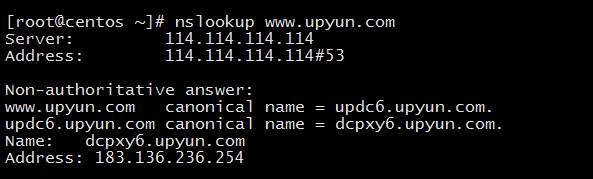
DNS series (I): why does the updated DNS record not take effect?
The strongest installation of the twin tower model, Google is playing "antique" again?
Preparing for the interview and sharing experience
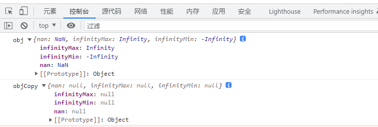
Use json Stringify() to realize deep copy, be careful, there may be a huge hole
![VTOL in Px4_ att_ Control source code analysis [supplement]](/img/7a/4ce0c939b9259faf59c52da2587693.jpg)
VTOL in Px4_ att_ Control source code analysis [supplement]
![[open source] Net ORM accessing Firebird database](/img/a2/4eff4f0af53bf3b9839a73019a212f.png)
[open source] Net ORM accessing Firebird database

随机推荐
戴森官方直营店免费造型服务现已开放预约 先锋科技诠释护发造型理念,助力消费者解锁多元闪耀造型
Antd date component appears in English
null == undefined
Px4 autonomous flight
Matplotlib快速入门
Where is the big data open source project, one-stop fully automated full life cycle operation and maintenance steward Chengying (background)?
The function is really powerful!
[azure microservice service fabric] start the performance monitor in the SF node and set the method of capturing the process
IP网络主动测评系统——X-Vision
Robot autonomous exploration series papers environment code
Latest Android advanced interview questions summary, Android interview questions and answers
使用 BlocConsumer 同时构建响应式组件和监听状态
如何选择合适的自动化测试工具?
Ren Qian code compilation error modification
海外代理推荐
[colmap] sparse reconstruction is converted to mvsnet format input
Reinforcement learning - learning notes 9 | multi step TD target
Revit secondary development - intercept project error / warning pop-up
SAR image quality evaluation
Gazebo import the mapping model created by blender