Import dependence
from tensorflow import keras
from matplotlib import pyplot as plt
from tensorflow.keras.layers import Conv2D, MaxPool2D, Flatten, Dense
Download datasets
mnist The dataset is a common set of handwritten numbers , Altogether 7W Zhang 28*28 Pixel point 0-9 Handwritten digital images and labels , Among them is 6W Zhang is a training set ,1W Zhang is a test set .
mnist = tf.keras.datasets.mnist
(x_train, y_train), (x_test, y_test) = mnist.load_data()
among ,x_train For training set features ,y_train Label the training set ,x_test For test set features ,y_test Label the test set .
Data normalization
Make it be 0-255 Between the gray values , Turn into 0-1 Value between , So that the gradient becomes smooth , It's easier to converge and find the optimal solution .
x_train, x_test = x_train / 255.0, x_test / 255.0
Increase the dimension
Add a dimension to the dataset , Turn it into 6W Zhang 28*28 Single channel data of , Let convolution kernel for feature extraction .
x_train = x_train.reshape(x_train.shape[0], 28, 28, 1)
x_test = x_test.reshape(x_test.shape[0], 28, 28, 1)
Hot code alone
y_train = keras.utils.to_categorical(y_train, 10)
y_test = keras.utils.to_categorical(y_test, 10)
After coding alone , Each category corresponds to a status code ,1 be for the purpose of ,0 Why not . If a picture tag is 6, The only hot code is :0 0 0 0 0 0 1 0 0 0
Split validation set
Take out of the training set 5000 Samples for verification set , The verification set is used to participate in training and update the gradient .
x_validation = x_train[:5000]
y_validation = y_train[:5000]
x_train = x_train[5000:]
y_train = y_train[5000:]
Build a network structure
Using three-layer convolution and two-layer fully connected network structure , The first layer of convolution uses 32 individual 3*3 Convolution kernel , The second and third layer convolution uses 64 individual 3*3 Convolution kernel , The purpose of convolution is to extract the spatial features of an image , Maximum pooling is to suppress over fitting .
model = keras.models.Sequential([
    Conv2D(32, (3, 3), activation='relu',input_shape=(28, 28, 1)),
    MaxPool2D((2, 2)),
    Conv2D(64, (3, 3), activation='relu'),
    MaxPool2D((2, 2)),
    Conv2D(64, (3, 3), activation='relu'),
    Flatten(),
    Dense(64, activation='relu'),
    Dense(10, activation='softmax')
])
Compile model
Using the cross entropy loss function of multi classification categories , Optimizer selection rmsprop, Under normal circumstances, you can choose this optimizer , It won't disappoint you , This is also the default optimizer .
model.compile(loss='categorical_crossentropy', optimizer='rmsprop',metrics=['accuracy'])
Save the model
checkpoint_save_path = "./checkpoint/mnist2.ckpt"
cp_callback = tf.keras.callbacks.ModelCheckpoint(filepath=checkpoint_save_path,save_weights_only=True, save_best_only=True)
Executive Training
Data set press 32 One is a batch feed neural network , Total iterations 7 Time , Test the accuracy once every iteration .
history = model.fit(x_train, y_train, batch_size=32, epochs=7, verbose=1, validation_data=(x_validation,y_validation),validation_freq=1,callbacks=[cp_callback])
Evaluation model
score = model.evaluate(x_test, y_test, verbose=0, batch_size=32)
print(' Test accuracy :{},  test loss value : {}'.format(score[1], score[0]))
visualization acc and loss curve
plt.rcParams['font.sans-serif']=['SimHei']
acc = history.history['accuracy']
val_acc = history.history['val_accuracy']
loss = history.history['loss']
val_loss = history.history['val_loss']

plt.subplot(1, 2, 1)
plt.plot(acc, label=' Training Acc')
plt.plot(val_acc, label=' test Acc')
plt.title('Acc curve ')
plt.legend()

plt.subplot(1, 2, 2)
plt.plot(loss, label=' Training Loss')
plt.plot(val_loss, label=' test Loss')
plt.title('Loss curve ')
plt.legend()
plt.show()
Now run the program , After training , The acc and loss Training image of , At the same time checkpoint Folder .
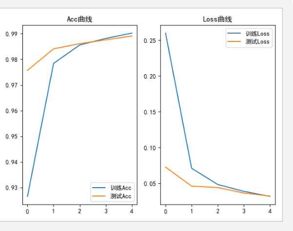
You can see , A neural network with convolution computation , The effect has been improved , The accuracy of the model test has reached 99%.
Reproduce the network structure
After training , Next, you should write an application , Used to receive pictures , Identify pictures , Return recognition results .
So I opened a new one here py file
from PIL import Image
import numpy as np
import tensorflow as tf
from tensorflow import keras
from tensorflow.keras.layers import Conv2D,  MaxPool2D, Flatten, Dense
First of all, we should reproduce the network structure of training
model = keras.models.Sequential([
    Conv2D(32, (3, 3), activation='relu',input_shape=(28, 28, 1)),
    MaxPool2D((2, 2)),
    Conv2D(64, (3, 3), activation='relu'),
    MaxPool2D((2, 2)),
    Conv2D(64, (3, 3), activation='relu'),
    Flatten(),
    Dense(64, activation='relu'),
    Dense(10, activation='softmax')
])
Load model
model_save_path = './checkpoint/mnist2.ckpt'
model.load_weights(model_save_path)
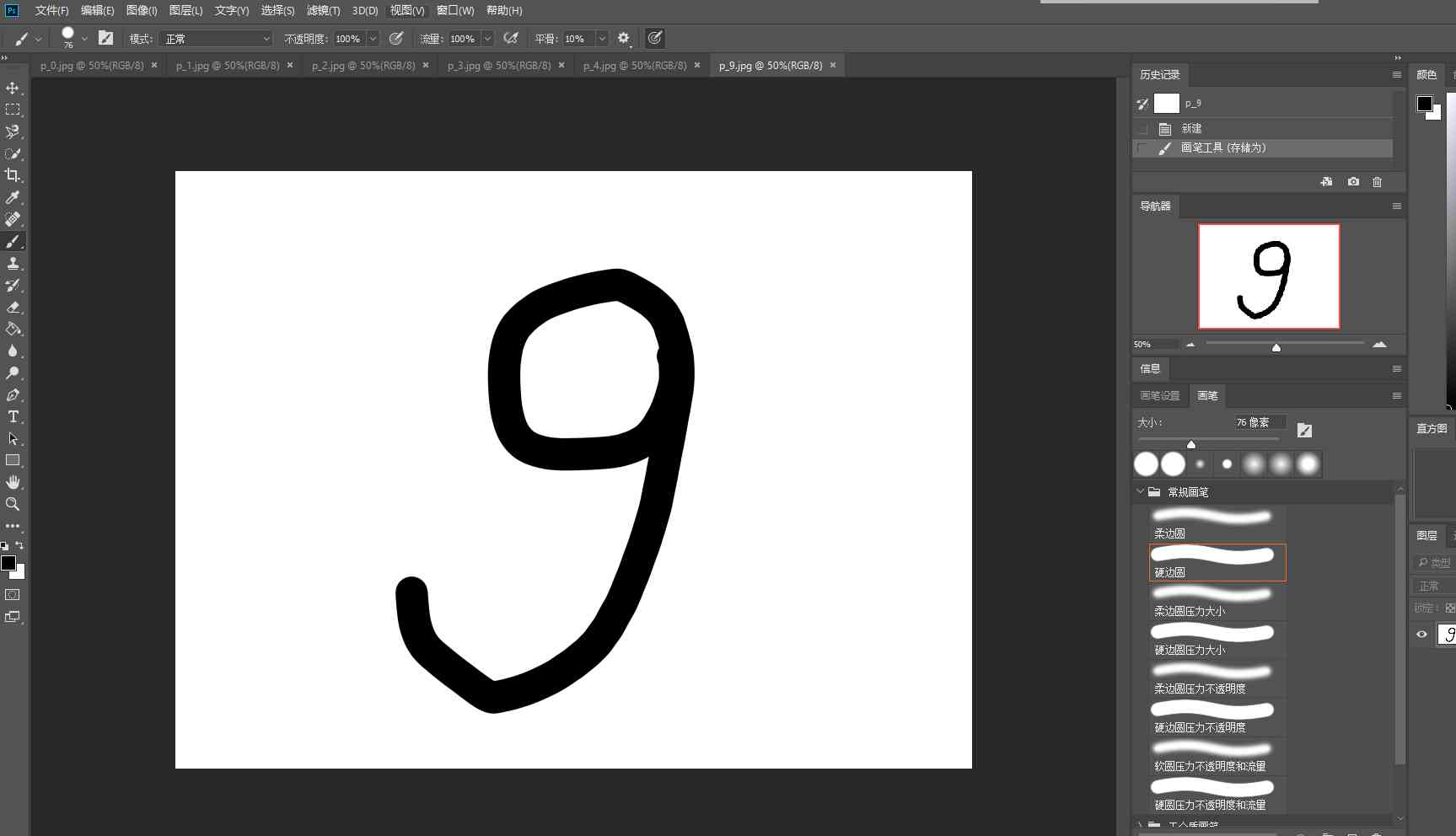
Image recognition
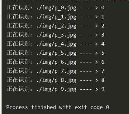
I use Photoshop I drew ten pictures , To identify
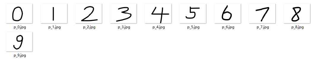
imgs = ['./img/p_0.jpg','./img/p_1.jpg','./img/p_2.jpg','./img/p_3.jpg','./img/p_4.jpg','./img/p_5.jpg','./img/p_6.jpg','./img/p_7.jpg','./img/p_8.jpg','./img/p_9.jpg']

for path in imgs:

    # Read the picture
    img = Image.open(path)
    img = img.resize((28, 28), Image.ANTIALIAS)
    img_arr = np.array(img.convert('L'))

    # The training picture is white on a black background , But the image we recognize is black on a white background , So we need color reversal
    # Converts the pixel value to 0 and 255 Two extremes   While retaining useful information in pictures   Filter out the background noise   Make the picture Cleaner
    for i in range(28):
        for j in range(28):
            if img_arr[i][j] < 150:
                img_arr[i][j] = 255
            else:
                img_arr[i][j] = 0

    #  normalization
    img_arr = img_arr / 255.0

    #  Add a dimension
    x_predict = img_arr.reshape(1, 28, 28, 1)

    #  distinguish
    result = model.predict(x_predict)
    pred = tf.argmax(result[0])
    print(' Identifying :{} ---- > {}'.format(path, pred))
Running results :

![[Python从零到壹] 五.网络爬虫之BeautifulSoup基础语法万字详解](/img/e8/dd70ddf3c2027907f64674676d676e.jpg)