当前位置：网站首页>Using lime to explain black box ML model

Using lime to explain black box ML model

2020-11-06 01:14:00 【Artificial intelligence meets pioneer】

flutter + Applet + Back end ,3 Individuals can open your APP The way | Registration will be sent to Dajiang Yuntai 、 Huawei watch ！>>>

author |Travis Tang (Voon Hao) compile |VK source |Towards Data Science

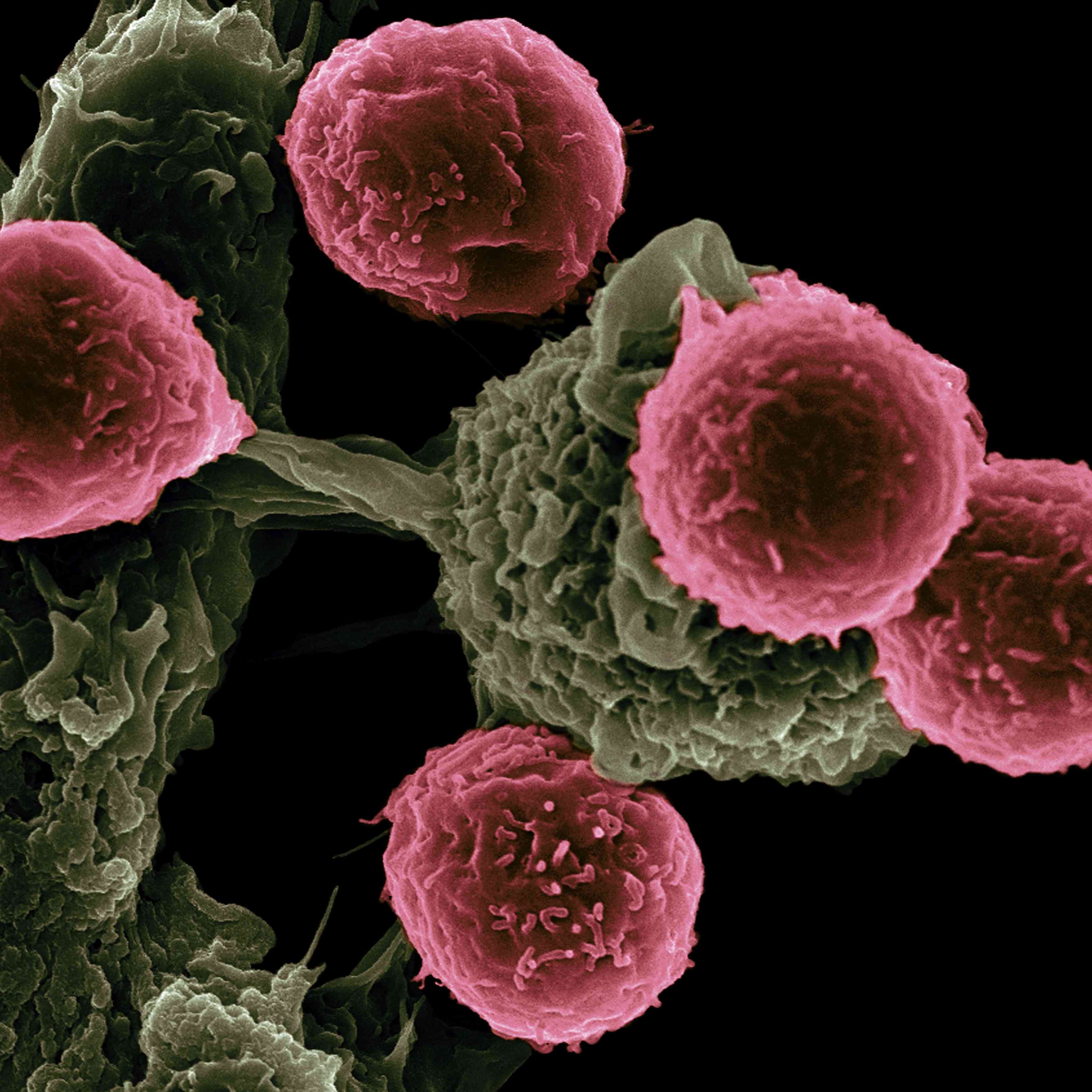
At this point , Anyone thinks that the potential of machine learning in medicine is a cliche . There are too many examples to support this statement - One of them is Microsoft's use of medical imaging data to help clinicians and radiologists make accurate cancer diagnoses . meanwhile , The development of advanced artificial intelligence algorithm greatly improves the accuracy of this kind of diagnosis . without doubt , Medical data is so amazing to use , There are good reasons to be excited about the benefits .

However , This cutting-edge algorithm is a black box , It may be difficult to explain . An example of the black box model is the deep neural network , After inputting data through millions of neurons in the network , Make a single decision . This black box model does not allow clinicians to use their prior knowledge and experience to verify the diagnosis of the model , Making model-based diagnostics less credible .

in fact , A recent survey of radiologists in Europe depicts a realistic picture of the use of black box models in radiology . The survey shows that , Only 55.4% Twenty percent of clinicians believe that there is no doctor's supervision , Patients will not accept pure artificial intelligence applications .[1]

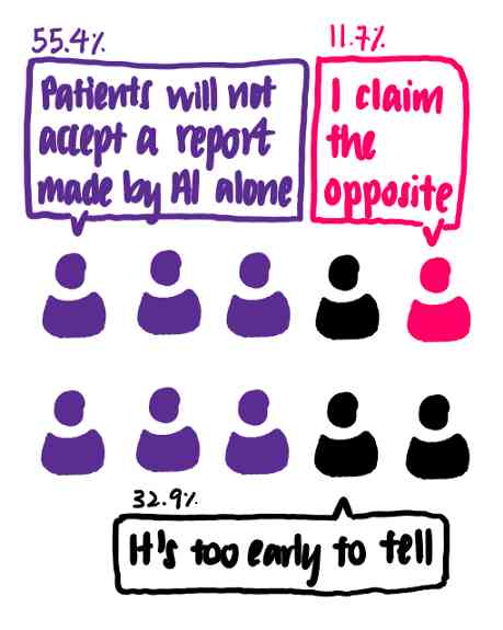
Under investigation 635 Of the doctors , More than half believed that patients were not ready to receive reports only generated by artificial intelligence .

The next question is ： If artificial intelligence can't completely replace the role of doctors , So how can artificial intelligence help doctors provide accurate diagnosis ？

This prompted me to explore existing solutions that help explain machine learning models . Generally speaking , Machine learning model can be divided into interpretable model and non interpretable model . In short , The output provided by an interpretable model is related to the importance of each input feature . Examples of these models include linear regression 、logistic Return to 、 Decision tree and decision rules, etc . On the other hand , Neural networks form a large number of unexplained models .

There are many solutions to help explain the black box model . These solutions include Shapley value 、 Partial dependence graphs and Local Interpretable Model Agnostic Explanations（LIME）, These methods are very popular among machine learning practitioners . today , I will focus on LIME.

according to Ribeiro wait forsomeone [2] Of LIME The paper ,LIME The goal is “ Identify an interpretable model that is locally faithful to the classifier on the interpretable representation ”. let me put it another way ,LIME Can explain the classification result of a specific point .LIME It also applies to all types of models , Make it independent of the model .

Intuitively explain LIME

It sounds hard to understand . Let's break it down step by step . Suppose we have the following toy dataset with two characteristics . Each data point is associated with a basic truth tag （ Positive or negative ） Related to .

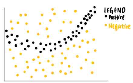
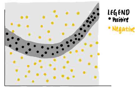
From the data points we can see that , Linear classifiers will not be able to recognize the boundary between positive and negative labels . therefore , We can train a nonlinear model , For example, neural networks , To classify these points . If the model is well trained , It can predict that new data points falling in the dark gray area will be positive , Another new data point in the light gray area is negative .

Now? , We're curious about the model for specific data points （ violet ） The decision made . We ask ourselves , Why is this particular point predicted by the neural network to be negative ？

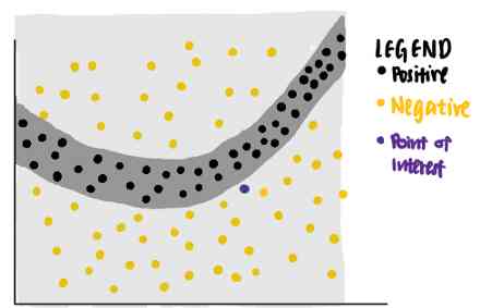
We can use LIME To answer this question .LIME First, random points are identified from the original data set , According to the distance between each data point and purple interest point, weight is assigned to each data point . The closer the sampled data point is to the point of interest , The more important it is .（ In the picture , A larger point means that the weight assigned to the data point is greater .）

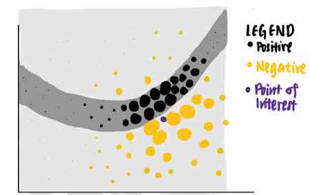
Use these points with different weights ,LIME An explanation with the highest interpretability and local fidelity is given .

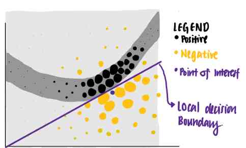
Use this standard ,LIME Identify the purple line as a known explanation for the point of interest . We can see , The purple line can explain that the decision boundary of neural network is close to the data point . The interpretation learned has a high local fidelity , But the overall fidelity is low .

Let's see LIME The role in practice ： Now? , I will focus on LIME The use of machine learning models in interpreting Wisconsin breast cancer data training .

Wisconsin breast cancer data set ： Understand the predictors of cancer cells

Wisconsin breast cancer data set [3], from UCI On 1992 Released in , contain 699 Data points . Each data point represents a cell sample , It can be malignant or benign . Each sample also has a number 1 To 10, For the following features .

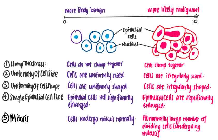
The thickness of the mass ：Clump Thickness
Cell size uniformity ：Uniformity of Cell Size
Cell shape uniformity ：Uniformity of Cell Shape
The size of a single epithelial cell ：Single Epithelial Cell Size
mitosis ：Mitoses
Normal nuclei ：Normal Nucleoli
Boring chromosomes ：Bland Chromatin
Naked core ：Bare Nuclei
Edge adhesion ：Marginal Adhesion

Let's try to understand what these features mean . The following illustration shows the difference between benign and malignant cells using the characteristics of the data set .

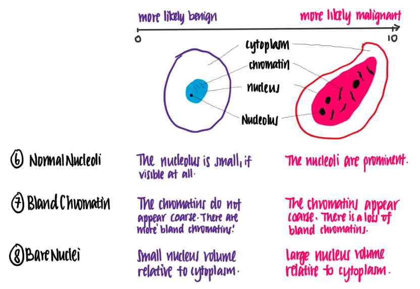
Thank you for your special lecture .

In this case , We can see that the higher each eigenvalue is , The more likely the cells are to be malignant .

Predicting whether a cell is malignant or benign

Now that we understand what data means , Let's start coding ！ We read the data first , Then clean up the data by deleting incomplete data points and reformatting class columns .

Data import 、 Clean up and explore

#  Data import and clean up 
import pandas as pd

df = pd.read_csv("/BreastCancerWisconsin.csv", 
                 dtype = 'float', header = 0)
df = df.dropna() #  Delete all rows that are missing values 

#  The original data set is in Class Use values in columns 2 and 4 To label benign and malignant cells . This code block formats it as a benign cell 0 class , Malignant cells are 1 class .

def reformat(value):
    if value == 2: 
        return 0 #  Benign 
    elif value == 4:
        return 1 #  Malignant 
        
df['Class'] = df.apply(lambda row: reformat(row['Class']), axis = 'columns')

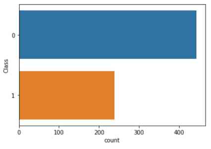
After deleting the incomplete data , We did a simple study of the data . By drawing cell sample categories （ Malignant or benign ） The distribution of , We found benign （0 level ） More cell samples than malignant （1 level ） Cell samples .

import seaborn as sns
sns.countplot(y='Class', data=df)

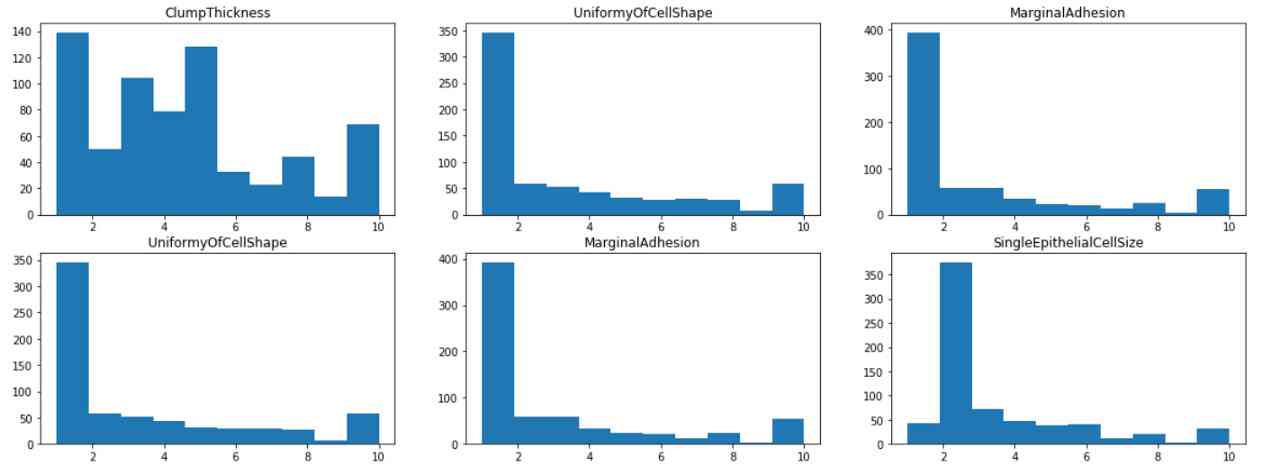
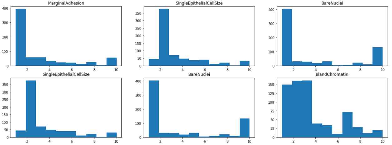
By visualizing the histogram of each feature , We found that most of the features have 1 or 2 The pattern of , Except for lumps and pastels , It is distributed in 1 To 10 More even between . This suggests that clump thickness and dull chromatin may be a weak predictor of this class .

from matplotlib import pyplot as plt
fig, axes = plt.subplots(4,3, figsize=(20,15))
for i in range(0,4):
    for j in range(0,3):
        axes[i,j].hist(df.iloc[:,1+i+j])
        axes[i,j].set_title(df.iloc[:,1+i+j].name)

Model training and testing

then , Press the dataset to 80%-10%-10% The proportion of training verification test set is divided into typical training verification test set , utilize Sklearn establish K- The nearest neighbor model . After some super parameter adjustment （ Not shown ）, Find out k=10 In the evaluation phase - its F1 The score is 0.9655. The code block looks like this .

from sklearn.model_selection import train_test_split
from sklearn.model_selection import KFold

#  Training test split 
X_traincv, X_test, y_traincv, y_test = train_test_split(data, target, test_size=0.1, random_state=42)

# K- Folding verification 
kf = KFold(n_splits=5, random_state=42, shuffle=True)

for train_index, test_index in kf.split(X_traincv):
    X_train, X_cv = X_traincv.iloc[train_index], X_traincv.iloc[test_index]
    y_train, y_cv = y_traincv.iloc[train_index], y_traincv.iloc[test_index]
    
from sklearn.neighbors import KNeighborsClassifier
from sklearn.metrics import f1_score,

#  Training KNN Model 
KNN = KNeighborsClassifier(k=10)
KNN.fit(X_train, y_train)

#  assessment KNN Model 
score =  f1_score(y_testset, y_pred, average="binary", pos_label = 4)
print ("{} => F1-Score is {}" .format(text, round(score,4)))

Use LIME The model explains

One Kaggle Experts might say that's a good result , We can do this project here . However , People should be skeptical about the decision of the model , Even if the model performs well in the evaluation . therefore , We use LIME To explain KNN The model's decision on this dataset . This verifies the validity of the model by checking whether the decision is in line with our intuition .

import lime
import lime.lime_tabular

# LIME Get ready 
predict_fn_rf = lambda x: KNN.predict_proba(x).astype(float)

#  Create a LIME Interpreter 
X = X_test.values
explainer = lime.lime_tabular.LimeTabularExplainer(X,feature_names =X_test.columns, class_names = ['benign','malignant'], kernel_width = 5)

#  Select the data points to interpret 
chosen_index = X_test.index[j]
chosen_instance = X_test.loc[chosen_index].values

#  Use LIME The interpreter interprets data points 
exp = explainer.explain_instance(chosen_instance, predict_fn_rf, num_features = 10)

exp.show_in_notebook(show_all=False)

ad locum , I chose 3 Point to illustrate LIME How it is used .

Explain why the sample is predicted to be malignant

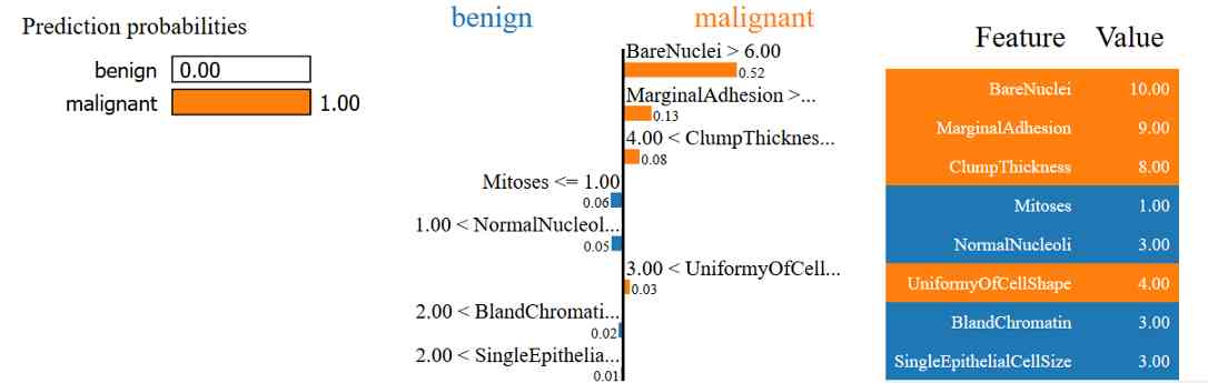
here , We have a data point , It's actually malignant , And it was predicted to be malignant . On the left panel , We see KNN The model predicts that this is close to 100% The probability is malignant . In the middle , We observed that LIME Be able to use every feature of a data point , Explain this prediction in order of importance . according to LIME That's what I'm saying ,

in fact , The value of the sample for the naked core is greater than 6.0, This makes it more likely to be malignant .
Because of the high edge adhesion of the sample , It's more likely to be malignant than benign .
Because the thickness of the sample is larger than 4, It's more likely to be malignant .
On the other hand , The mitotic value of the sample ≤1.00 This fact makes it more likely to be benign .

in general , Considering all the characteristics of the sample （ On the right panel ）, The sample was predicted to be malignant .

These four observations are consistent with our intuition and understanding of cancer cells . Knowing that , We believe that models make the right predictions based on our intuition . Let's look at another example .

Explain why predictive samples are benign

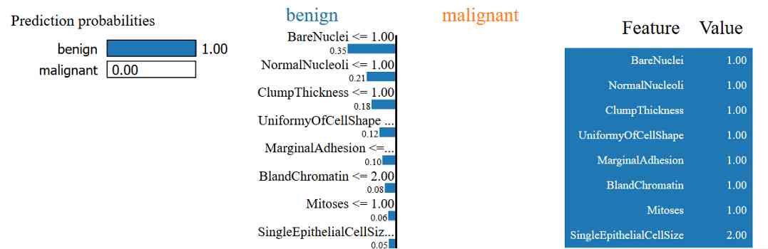
ad locum , We have a sample cell , Predictions are benign , It's actually benign .LIME By quoting （ Among other reasons ） Explains why this happens

The bare core value of the sample is ≤1
The normal value of nucleolus of this sample ≤1
Its mass thickness is also ≤1
The shape of the cells is also uniform ≤1

Again , These are in line with our intuition about why cells are benign .

Explain why the sample predictions are not clear

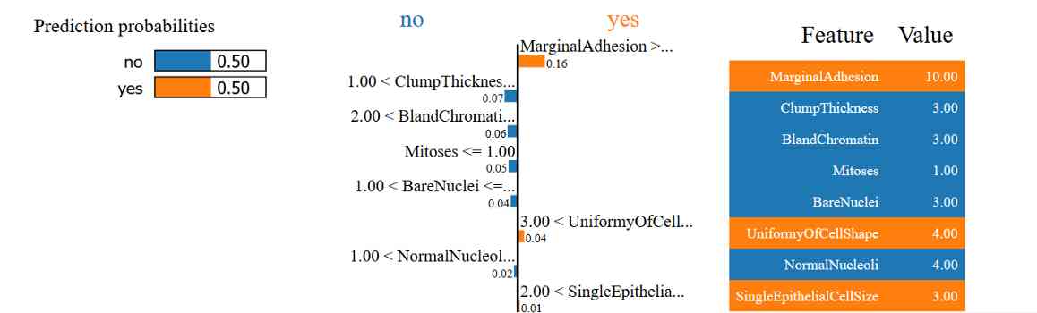
In the last example , We see that this model can't predict whether cells are benign or malignant . You can use LIME Do you understand why this happened ？

Conclusion

LIME From tabular data to text and images , Make it incredibly versatile . However , There is still work to be done . for example , The author of this paper holds that , The current algorithm is too slow to apply to images , It doesn't work .

For all that , In terms of bridging the gap between the usefulness and the intractability of the black box model ,LIME Still very useful . If you want to start using LIME, A good starting point is LIME Of Github page .