当前位置:网站首页>Numerical calculation method chapter8 Numerical solutions of ordinary differential equations
Numerical calculation method chapter8 Numerical solutions of ordinary differential equations
2022-07-05 17:59:00 【Espresso Macchiato】
- Numerical calculation method Chapter8. Numerical solutions of ordinary differential equations
0. Problem description
The problems examined in this chapter are described in the title , That is, the numerical solution of ordinary differential equations :
{ d y d x = f ( x , y ) y ( x 0 ) = y 0 \left\{ \begin{aligned} \frac{dy}{dx} &= f(x, y) \\ y(x_0) &= y_0 \end{aligned} \right. ⎩⎨⎧dxdyy(x0)=f(x,y)=y0
1. Euler The formula
1. forward Euler The formula
Euler Formula is a relatively direct way to solve the numerical solution of ordinary differential equations :
d y d x = δ y δ x = f ( x , y ) \frac{dy}{dx} = \frac{\delta y}{\delta x} = f(x, y) dxdy=δxδy=f(x,y)
Thus there are :
y + δ y = f ( x , y ) ⋅ δ x y+\delta y = f(x, y) \cdot \delta x y+δy=f(x,y)⋅δx
thus , We can approximate each by constantly solving x x x Value under y y y value .
y n + 1 = y n + h ⋅ f ( x n , y n ) y_{n+1} = y_n + h\cdot f(x_n, y_n) yn+1=yn+h⋅f(xn,yn)
give python The pseudo code is implemented as follows :
def fwd_euler_fn(f, x0, y0, step=1e-3):
    def fn(x):
        h = step if x >= x0 else -step
        n = math.ceil((x - x0) / h)
        x, y = x0, y0
        for _ in range(n):
            y += h * f(x, y)
            x += h
        return y
    return fn
2. backward Euler The formula
backward Euler Formula and forward Euler There is no essential difference between formulas , However, the fine-tuning formula is :
y n + 1 = y n + h ⋅ f ( x n + 1 , y n + 1 ) y_{n+1} = y_n + h\cdot f(x_{n+1}, y_{n+1}) yn+1=yn+h⋅f(xn+1,yn+1)
But it's obviously calculating y n + 1 y_{n+1} yn+1 In fact, I can't know f ( x n + 1 , y n + 1 ) f(x_{n+1}, y_{n+1}) f(xn+1,yn+1) Value , Therefore, we need to superimpose the idea of iteration :
y n + 1 ( k + 1 ) = y n ( k + 1 ) + h ⋅ f ( x n + 1 , y n + 1 ( k ) ) y_{n+1}^{(k+1)} = y_n^{(k+1)} + h\cdot f(x_{n+1}, y_{n+1}^{(k)}) yn+1(k+1)=yn(k+1)+h⋅f(xn+1,yn+1(k))
The above iterative formula is called Picard iteration .
Can prove that , When h h h Enough hours ,Picard Iterative convergence .
give python The pseudocode is as follows :
def bwd_euler_fn(f, x0, y0, step=1e-3):
    def fn(x, epsilon = 1e-6):
        h = step if x >= x0 else -step
        n = math.ceil((x - x0) / h)
        xlist = [x0 + i*h for i in range(n)]
        ylist = [y0 for i in range(n)]
        for i in range(n-1):
            ylist[i+1] = ylist[i] + h * f(xlist[i], ylist[i])
        while True:
            zlist = deepcopy(ylist)
            for i in range(n-1):
                zlist[i+1] = zlist[i] + h * f(xlist[i+1], ylist[i+1])
            delta = abs(zlist[-1] - ylist[-1])
            ylist = zlist
            if delta < epsilon:
                break
        return zlist[-1]
    return fn
3. Trapezoidal formula
Trapezoidal formula is still based on differential difference quotient in essence , However, it is different from the direct use of differentiation before , The expression of integral is used more strictly here , namely :
y n + 1 = y n + ∫ x n x n + 1 f ( x , y ) d x y_{n+1} = y_n + \int_{x_{n}}^{x_{n+1}}f(x, y)dx yn+1=yn+∫xnxn+1f(x,y)dx
then , Here the trapezoidal formula is used to approximate the integration process , Yes :
y n + 1 = y n + h 2 ( f ( x n , y n ) + f ( x n + 1 , y n + 1 ) ) y_{n+1} = y_n + \frac{h}{2}(f(x_n, y_n) + f(x_{n+1}, y_{n+1})) yn+1=yn+2h(f(xn,yn)+f(xn+1,yn+1))
Here we will also refer to y n + 1 y_{n+1} yn+1 The solution of the problem , however , Different from backward Euler The pure iterative idea in the formula , Only one iteration is used here to approximate , namely :
y n + 1 = y n + h 2 ( f ( x n , y n ) + f ( x n + 1 , y n + h ⋅ f ( x n , y n ) ) ) y_{n+1} = y_n + \frac{h}{2}(f(x_n, y_n) + f(x_{n+1}, y_{n} + h\cdot f(x_n, y_n))) yn+1=yn+2h(f(xn,yn)+f(xn+1,yn+h⋅f(xn,yn)))
Again , We give python The pseudo code is implemented as follows :
def tapezoid_fn(f, x0, y0, step=1e-3):
    def fn(x):
        h = step if x >= x0 else -step
        n = math.ceil((x - x0) / h)
        x, y = x0, y0
        for _ in range(n):
            y += h/2 * (f(x, y) + f(x+h, y+h*f(x, y)))
            x += h
        return y
    return fn
2. Runge-Kutta Method
1. Second order Runge-Kutta Method
Runge-Kutta Compared with the previous Euler Formula is a method with relatively higher accuracy .
Euler The formula comes from the definition of differential , and Runge-Kutta The method investigated Taylor an , Yes :
y n + 1 = y n + ∑ i h i i ! y ( i ) ( x n ) = y n + h ⋅ y ′ ( x n ) + h 2 2 ! ⋅ y ′ ′ ( x n ) + . . . \begin{aligned} y_{n+1} &= y_n + \sum_{i} \frac{h^i}{i!} y^{(i)}(x_n) \\ &= y_n + h \cdot y'(x_n) + \frac{h^2}{2!} \cdot y''(x_n) + ... \end{aligned} yn+1=yn+i∑i!hiy(i)(xn)=yn+h⋅y′(xn)+2!h2⋅y′′(xn)+...
We keep the second-order term, that is :
y n + 1 = y n + h ⋅ y ′ ( x n ) + h 2 2 y ′ ′ ( x n ) = y n + h ⋅ f ( x n , y n ) + h 2 2 ( ∂ f ∂ x ( x n , y n ) + ∂ f ∂ y ( x n , y n ) ⋅ f ( x n , y n ) ) \begin{aligned} y_{n+1} &= y_n + h \cdot y'(x_n) + \frac{h^2}{2} y''(x_n) \\ &= y_n + h \cdot f(x_n, y_n) + \frac{h^2}{2}(\frac{\partial f}{\partial x}(x_n, y_n) + \frac{\partial f}{\partial y}(x_n, y_n) \cdot f(x_n, y_n)) \end{aligned} yn+1=yn+h⋅y′(xn)+2h2y′′(xn)=yn+h⋅f(xn,yn)+2h2(∂x∂f(xn,yn)+∂y∂f(xn,yn)⋅f(xn,yn))
however , One problem here is that the two partial derivatives are not necessarily easy to solve , Therefore, the above expression cannot be called directly .
and Runge-Kutta The method is to use an approximate displacement formula to estimate it , So that there is no error between them in the second derivative range .
To be specific :
Δ = y n + − y n = h ⋅ y ′ ( x n ) + h 2 2 y ′ ′ ( x n ) = h ⋅ f ( x n , y n ) + h 2 2 ( ∂ f ∂ x ( x n , y n ) + ∂ f ∂ y ( x n , y n ) ⋅ f ( x n , y n ) ) = c 1 ⋅ h ⋅ f ( x n , y n ) + c 2 ⋅ h ⋅ f ( x n + a h , y n + b h f ( x n , y n ) ) = c 1 ⋅ h ⋅ f ( x n , y n ) + c 2 ⋅ h ⋅ [ f ( x n , y n ) + ∂ f ∂ x ( x n , y n ) ⋅ a h + ∂ f ∂ y ( x n , y n ) ⋅ b h f ( x n , y n ) ] \begin{aligned} \Delta &= y_{n+} - y_n \\ &= h \cdot y'(x_n) + \frac{h^2}{2} y''(x_n) \\ &= h \cdot f(x_n, y_n) + \frac{h^2}{2}(\frac{\partial f}{\partial x}(x_n, y_n) + \frac{\partial f}{\partial y}(x_n, y_n) \cdot f(x_n, y_n)) \\ &= c_1\cdot h\cdot f(x_n, y_n) + c_2 \cdot h \cdot f(x_n + ah, y_n + bhf(x_n, y_n)) \\ &= c_1 \cdot h \cdot f(x_n, y_n) + c_2 \cdot h \cdot [f(x_n, y_n) + \frac{\partial f}{\partial x}(x_n, y_n) \cdot ah + \frac{\partial f}{\partial y}(x_n, y_n) \cdot bhf(x_n, y_n)] \end{aligned} Δ=yn+−yn=h⋅y′(xn)+2h2y′′(xn)=h⋅f(xn,yn)+2h2(∂x∂f(xn,yn)+∂y∂f(xn,yn)⋅f(xn,yn))=c1⋅h⋅f(xn,yn)+c2⋅h⋅f(xn+ah,yn+bhf(xn,yn))=c1⋅h⋅f(xn,yn)+c2⋅h⋅[f(xn,yn)+∂x∂f(xn,yn)⋅ah+∂y∂f(xn,yn)⋅bhf(xn,yn)]
Or say , Give parameters c 1 , c 2 , a , b c_1, c_2, a, b c1,c2,a,b Make the following conditions meet :
{ y n + 1 = y n + h ( c 1 ⋅ k 1 + c 2 ⋅ k 2 ) k 1 = f ( x n , y n ) k 2 = f ( x n + a h , y n + b h k 1 ) \left\{ \begin{aligned} y_{n+1} &= y_n + h(c_1 \cdot k_1 + c_2 \cdot k_2) \\ k_1 &= f(x_n, y_n) \\ k_2 &= f(x_n + ah, y_n + bhk_1) \end{aligned} \right. ⎩⎪⎨⎪⎧yn+1k1k2=yn+h(c1⋅k1+c2⋅k2)=f(xn,yn)=f(xn+ah,yn+bhk1)
bring y n + 1 y_{n+1} yn+1 There is no error in the range of the second derivative .
or :
{ ( c 1 + c 2 ) h ⋅ f ( x n , y n ) = h c 2 a h 2 ⋅ ∂ f ∂ x ( x n , y n ) = h 2 2 ∂ f ∂ x ( x n , y n ) c 2 b h 2 ⋅ ∂ f ∂ y ( x n , y n ) = h 2 2 ∂ f ∂ y ( x n , y n ) \left\{ \begin{aligned} (c_1 + c_2)h \cdot f(x_n, y_n) &= h \\ c_2 a h^2 \cdot \frac{\partial f}{\partial x}(x_n, y_n) &= \frac{h^2}{2} \frac{\partial f}{\partial x}(x_n, y_n) \\ c_2 b h^2 \cdot \frac{\partial f}{\partial y}(x_n, y_n) &= \frac{h^2}{2} \frac{\partial f}{\partial y}(x_n, y_n) \end{aligned} \right. ⎩⎪⎪⎪⎪⎪⎨⎪⎪⎪⎪⎪⎧(c1+c2)h⋅f(xn,yn)c2ah2⋅∂x∂f(xn,yn)c2bh2⋅∂y∂f(xn,yn)=h=2h2∂x∂f(xn,yn)=2h2∂y∂f(xn,yn)
Simplify the above formula to get :
{ c 1 + c 2 = 1 2 c 2 a = 1 2 c 2 b = 1 \left\{ \begin{aligned} c_1 + c_2 &= 1 \\ 2c_2 a &= 1 \\ 2c_2 b &= 1 \end{aligned} \right. ⎩⎪⎨⎪⎧c1+c22c2a2c2b=1=1=1
As long as the above equations are satisfied , The corresponding parameter a , b , c 1 , c 2 a,b,c_1,c_2 a,b,c1,c2 Both of them can make the above two formulas have no error within the second derivative range .
Give two groups of common second order Runge-Kutta The formula is as follows :
c 1 = 1 2 , c 2 = 1 2 , a = 1 , b = 1 c_1=\frac{1}{2}, c_2=\frac{1}{2}, a=1, b=1 c1=21,c2=21,a=1,b=1
{ k 1 = f ( x n , y n ) k 2 = f ( x n + h , y n + h k 1 ) y n + 1 = y n + h 2 ( k 1 + k 2 ) \left\{ \begin{aligned} k_1 &= f(x_n, y_n) \\ k_2 &= f(x_n + h, y_n + hk_1) \\ y_{n+1} &= y_n + \frac{h}{2}(k_1 + k_2) \end{aligned} \right. ⎩⎪⎪⎪⎨⎪⎪⎪⎧k1k2yn+1=f(xn,yn)=f(xn+h,yn+hk1)=yn+2h(k1+k2)
c 1 = 0 , c 2 = 1 , a = 1 2 , b = 1 2 c_1=0, c_2=1, a=\frac{1}{2}, b=\frac{1}{2} c1=0,c2=1,a=21,b=21
{ k 1 = f ( x n , y n ) k 2 = f ( x n + h 2 , y n + h 2 k 1 ) y n + 1 = y n + h k 2 \left\{ \begin{aligned} k_1 &= f(x_n, y_n) \\ k_2 &= f(x_n + \frac{h}{2}, y_n + \frac{h}{2}k_1) \\ y_{n+1} &= y_n + hk_2 \end{aligned} \right. ⎩⎪⎪⎪⎨⎪⎪⎪⎧k1k2yn+1=f(xn,yn)=f(xn+2h,yn+2hk1)=yn+hk2
2. Higher order Runge-Kutta Method
alike , We follow the above ideas , Give the general higher order Runge-Kutta The expression of the method is as follows :
{ y n + 1 = y n + h ( c 1 ⋅ k 1 + c 2 ⋅ k 2 + . . . + c m ⋅ k m ) k 1 = f ( x n , y n ) k 2 = f ( x n + a 1 h + y n + b 1 , 1 h ⋅ k 1 ) . . . k m = f ( x n + a m − 1 h + y n + ∑ i = 1 m − 1 b m − 1 , i h ⋅ k i ) \left\{ \begin{aligned} y_{n+1} &= y_n + h(c_1 \cdot k_1 + c_2 \cdot k_2 + ... + c_m \cdot k_m) \\ k_1 &= f(x_n, y_n) \\ k_2 &= f(x_n + a_{1} h + y_n + b_{1,1} h \cdot k_1) \\ &... \\ k_m &= f(x_n + a_{m-1} h + y_n + \sum_{i=1}^{m-1}b_{m-1,i} h \cdot k_{i}) \end{aligned} \right. ⎩⎪⎪⎪⎪⎪⎪⎪⎪⎪⎨⎪⎪⎪⎪⎪⎪⎪⎪⎪⎧yn+1k1k2km=yn+h(c1⋅k1+c2⋅k2+...+cm⋅km)=f(xn,yn)=f(xn+a1h+yn+b1,1h⋅k1)...=f(xn+am−1h+yn+i=1∑m−1bm−1,ih⋅ki)
Parameters a , b , c a,b,c a,b,c You can make y n y_n yn have O ( h m + 1 ) O(h^{m+1}) O(hm+1) Order accuracy .
or ,Taylor Expand until h m h^{m} hm Both sides have the same expansion coefficient .
1. Third order Runge-Kutta Method
We give the third order Runge-Kutta Two sets of typical coefficients of the method are as follows :
Coefficient combination ( One )
{ y n + 1 = y n + h 6 ( k 1 + 4 k 2 + k 3 ) k 1 = f ( x n , y n ) k 2 = f ( x n + 1 2 h , y n + 1 2 h k 1 ) k 3 = f ( x n + h , y n − h k 1 + 2 h k 2 ) \left\{ \begin{aligned} y_{n+1} &= y_n + \frac{h}{6}(k_1 + 4k_2 + k_3) \\ k_1 &= f(x_n, y_n) \\ k_2 &= f(x_n + \frac{1}{2}h, y_n + \frac{1}{2}hk_1) \\ k_3 &= f(x_n + h, y_n - hk_1 + 2hk_2) \end{aligned} \right. ⎩⎪⎪⎪⎪⎪⎪⎨⎪⎪⎪⎪⎪⎪⎧yn+1k1k2k3=yn+6h(k1+4k2+k3)=f(xn,yn)=f(xn+21h,yn+21hk1)=f(xn+h,yn−hk1+2hk2)
Coefficient combination ( Two )
{ y n + 1 = y n + h 4 ( k 1 + 3 k 3 ) k 1 = f ( x n , y n ) k 2 = f ( x n + 1 3 h , y n + 1 3 h k 1 ) k 3 = f ( x n + 2 3 h , y n + 2 3 h k 2 ) \left\{ \begin{aligned} y_{n+1} &= y_n + \frac{h}{4}(k_1 + 3k_3) \\ k_1 &= f(x_n, y_n) \\ k_2 &= f(x_n + \frac{1}{3}h, y_n + \frac{1}{3}hk_1) \\ k_3 &= f(x_n + \frac{2}{3}h, y_n + \frac{2}{3}hk_2) \end{aligned} \right. ⎩⎪⎪⎪⎪⎪⎪⎪⎪⎨⎪⎪⎪⎪⎪⎪⎪⎪⎧yn+1k1k2k3=yn+4h(k1+3k3)=f(xn,yn)=f(xn+31h,yn+31hk1)=f(xn+32h,yn+32hk2)
Coefficient combination ( 3、 ... and )
{ y n + 1 = y n + h 9 ( 2 k 1 + 3 k 2 + 4 k 3 ) k 1 = f ( x n , y n ) k 2 = f ( x n + 1 2 h , y n + 1 2 h k 1 ) k 3 = f ( x n + 3 4 h , y n + 3 4 h k 2 ) \left\{ \begin{aligned} y_{n+1} &= y_n + \frac{h}{9}(2k_1 + 3k_2 + 4k_3) \\ k_1 &= f(x_n, y_n) \\ k_2 &= f(x_n + \frac{1}{2}h, y_n + \frac{1}{2}hk_1) \\ k_3 &= f(x_n + \frac{3}{4}h, y_n + \frac{3}{4}hk_2) \end{aligned} \right. ⎩⎪⎪⎪⎪⎪⎪⎪⎪⎨⎪⎪⎪⎪⎪⎪⎪⎪⎧yn+1k1k2k3=yn+9h(2k1+3k2+4k3)=f(xn,yn)=f(xn+21h,yn+21hk1)=f(xn+43h,yn+43hk2)
2. Four order Runge-Kutta Method
alike , We can give two groups of typical fourth order Runge-Kutta The formula is as follows :
Coefficient combination ( One )
{ y n + 1 = y n + h 6 ( k 1 + 2 k 2 + 2 k 3 + k 4 ) k 1 = f ( x n , y n ) k 2 = f ( x n + 1 2 h , y n + 1 2 h k 1 ) k 3 = f ( x n + 1 2 h , y n + 1 2 h k 2 ) k 4 = f ( x n + h , y n + h k 3 ) \left\{ \begin{aligned} y_{n+1} &= y_n + \frac{h}{6}(k_1 + 2k_2 + 2k_3 + k_4) \\ k_1 &= f(x_n, y_n) \\ k_2 &= f(x_n + \frac{1}{2}h, y_n + \frac{1}{2}hk_1) \\ k_3 &= f(x_n + \frac{1}{2}h, y_n + \frac{1}{2}hk_2) \\ k_4 &= f(x_n + h, y_n + hk_3) \end{aligned} \right. ⎩⎪⎪⎪⎪⎪⎪⎪⎪⎪⎪⎨⎪⎪⎪⎪⎪⎪⎪⎪⎪⎪⎧yn+1k1k2k3k4=yn+6h(k1+2k2+2k3+k4)=f(xn,yn)=f(xn+21h,yn+21hk1)=f(xn+21h,yn+21hk2)=f(xn+h,yn+hk3)
Coefficient combination ( Two )
{ y n + 1 = y n + h 8 ( k 1 + 3 k 2 + 3 k 3 + k 4 ) k 1 = f ( x n , y n ) k 2 = f ( x n + 1 3 h , y n + 1 3 h k 1 ) k 3 = f ( x n + 2 3 h , y n + 1 3 h k 1 + h k 2 ) k 4 = f ( x n + h , y n + h k 1 − h k 2 + h k 3 ) \left\{ \begin{aligned} y_{n+1} &= y_n + \frac{h}{8}(k_1 + 3k_2 + 3k_3 + k_4) \\ k_1 &= f(x_n, y_n) \\ k_2 &= f(x_n + \frac{1}{3}h, y_n + \frac{1}{3}hk_1) \\ k_3 &= f(x_n + \frac{2}{3}h, y_n + \frac{1}{3}hk_1 + hk_2) \\ k_4 &= f(x_n + h, y_n + hk_1 - hk_2 + hk_3) \end{aligned} \right. ⎩⎪⎪⎪⎪⎪⎪⎪⎪⎪⎪⎨⎪⎪⎪⎪⎪⎪⎪⎪⎪⎪⎧yn+1k1k2k3k4=yn+8h(k1+3k2+3k3+k4)=f(xn,yn)=f(xn+31h,yn+31hk1)=f(xn+32h,yn+31hk1+hk2)=f(xn+h,yn+hk1−hk2+hk3)
3. python Pseudo code implementation
below , Let's give Runge-Kutta Methodical python The pseudo code is implemented as follows :
def runge_kutta_fn(f, x0, y0, a, b, c, step=1e-3):
    def fn(x):
        h = step if x >= x0 else -step
        n = math.ceil((x - x0) / h)
        m = len(c)
        assert(len(a) == m-1 and all(len(b[i]) == i+1 for i in range(m-1)))
        k = [0 for _ in range(m)]
        x, y = x0, y0
        for _ in range(n):
            k[0] = f(x, y)
            for i in range(m-1):
                xi = x + a[i] * h
                yi = y
                for j in range(i+1):
                    yi += h * b[i][j] * k[j]
                k[i+1] = f(xi, yi)
            x += h
            y += sum(ci * ki * h for ci, ki in zip(c, k))
        return y
    return fn
3. Linear multistep method
1. The basic idea
The idea source of linear multistep method is still integral formula :
y ( x ) = y ( x 0 ) + ∫ x 0 x y ′ ( t ) d t y(x) = y(x_0) + \int_{x_0}^{x}y'(t)dt y(x)=y(x0)+∫x0xy′(t)dt
Before ,Euler Formula and Runge-Kutta The method is to estimate the value of the integral directly .
among ,Euler The formula is direct ∫ x x + h y ′ ( t ) d t = y ′ ( x ) h \int_{x}^{x+h}y'(t)dt = y'(x)h ∫xx+hy′(t)dt=y′(x)h, and Runge-Kutta The method is to introduce a series of offsets to make y ( x ) y(x) y(x) stay n n n rank Taylor There is no error in expansion .
The approximate idea of linear multistep method is the idea of using the previous interpolation formula , Come on y ′ ( x ) y'(x) y′(x) To fit , Then use this fitting function to calculate the following integral value .
The description in the book is as follows :
If you use the integral node x n , x n − 1 , . . . , x n − q x_n, x_{n-1}, ..., x_{n-q} xn,xn−1,...,xn−q Construct interpolation polynomial approximation y ′ ( x ) y'(x) y′(x), In the interval [ x n − p , x n + 1 ] [x_{n-p}, x_{n+1}] [xn−p,xn+1] Calculate numerical integration on ∫ x n − p x n + 1 y ′ ( x ) d x \int_{x_{n-p}}^{x_{n+1}}y'(x)dx ∫xn−pxn+1y′(x)dx, Then it is called structural calculation y n + 1 y_{n+1} yn+1 The method is linear multistep .
Special :
- If you use x n , x n − 1 , . . . , x n − q x_{n}, x_{n-1}, ..., x_{n-q} xn,xn−1,...,xn−q Construct interpolation polynomials , Then the fitting function is called explicit Adams The formula ;
- If you use x n + 1 , x n , . . . , x n + 1 − q x_{n+1}, x_{n}, ..., x_{n+1-q} xn+1,xn,...,xn+1−q Construct interpolation polynomials , Then the fitting function is called implicit Admas The formula ;
2. Adams The formula
here , Let's not deduce , Directly give some common Adams The formula is as follows :
Second order explicit Adams The formula
y n + 1 = y n + h 2 ( 3 f ( x n , y n ) − f ( x n − 1 , y n − 1 ) ) y_{n+1} = y_{n} + \frac{h}{2}(3f(x_{n}, y_{n}) - f(x_{n-1}, y_{n-1})) yn+1=yn+2h(3f(xn,yn)−f(xn−1,yn−1))
Second order implicit Adams The formula
y n + 1 = y n + h 2 ( f ( x n , y n ) + f ( x n + 1 , y n + 1 ) ) y_{n+1} = y_{n} + \frac{h}{2}(f(x_{n}, y_{n}) + f(x_{n+1}, y_{n+1})) yn+1=yn+2h(f(xn,yn)+f(xn+1,yn+1))
Third order display Adams The formula
y n + 1 = y n + h 12 ( 23 f ( x n , y n ) − 16 f ( x n − 1 , y n − 1 ) + 5 f ( x n − 2 , y n − 2 ) ) y_{n+1} = y_{n} + \frac{h}{12}(23f(x_{n}, y_{n}) - 16f(x_{n-1}, y_{n-1}) + 5f(x_{n-2}, y_{n-2})) yn+1=yn+12h(23f(xn,yn)−16f(xn−1,yn−1)+5f(xn−2,yn−2))
Third order implicit Adams The formula
y n + 1 = y n + h 12 ( 5 f ( x n + 1 , y n + 1 + 8 f ( x n , y n ) − f ( x n − 1 , y n − 1 ) ) y_{n+1} = y_{n} + \frac{h}{12}(5f(x_{n+1}, y_{n+1} + 8f(x_{n}, y_{n}) - f(x_{n-1}, y_{n-1})) yn+1=yn+12h(5f(xn+1,yn+1+8f(xn,yn)−f(xn−1,yn−1))
Fourth order explicit Adams The formula
y n + 1 = y n + h 24 ( 55 f ( x n , y n ) − 59 f ( x n − 1 , y n − 1 ) + 37 f ( x n − 2 , y n − 2 ) − 9 f ( x n − 3 , y n − 3 ) ) y_{n+1} = y_{n} + \frac{h}{24}(55f(x_{n}, y_{n}) - 59f(x_{n-1}, y_{n-1}) + 37f(x_{n-2}, y_{n-2}) - 9f(x_{n-3}, y_{n-3})) yn+1=yn+24h(55f(xn,yn)−59f(xn−1,yn−1)+37f(xn−2,yn−2)−9f(xn−3,yn−3))
Fourth order implicit Adams The formula
y n + 1 = y n + h 24 ( 9 f ( x n + 1 , y n + 1 + 19 f ( x n , y n ) − 5 f ( x n − 1 , y n − 1 ) + f ( x n − 2 , y n − 2 ) ) y_{n+1} = y_{n} + \frac{h}{24}(9f(x_{n+1}, y_{n+1} + 19f(x_{n}, y_{n}) - 5f(x_{n-1}, y_{n-1}) + f(x_{n-2}, y_{n-2})) yn+1=yn+24h(9f(xn+1,yn+1+19f(xn,yn)−5f(xn−1,yn−1)+f(xn−2,yn−2))
4. Numerical solution of ordinary differential equations
1. Numerical solution of first order ordinary differential equations
We give the expression of the initial value problem of the first order ordinary differential equation as follows :
{ d y 1 d x = f 1 ( x , y 1 , y 2 , . . . , y m ) d y 2 d x = f 2 ( x , y 1 , y 2 , . . . , y m ) . . . d y m d x = f m ( x , y 1 , y 2 , . . . , y m ) y 1 ( x 0 ) = η 1 y 2 ( x 0 ) = η 2 . . . y m ( x 0 ) = η m \left\{ \begin{aligned} \frac{dy_{1}}{dx} &= f_1(x, y_{1}, y_{2}, ..., y_{m}) \\ \frac{dy_{2}}{dx} &= f_2(x, y_{1}, y_{2}, ..., y_{m}) \\ &... \\ \frac{dy_{m}}{dx} &= f_m(x, y_{1}, y_{2}, ..., y_{m}) \\ y_1(x_0) &= \eta_1 \\ y_2(x_0) &= \eta_2 \\ &... \\ y_m(x_0) &= \eta_m \\ \end{aligned} \right. ⎩⎪⎪⎪⎪⎪⎪⎪⎪⎪⎪⎪⎪⎪⎪⎪⎪⎪⎪⎨⎪⎪⎪⎪⎪⎪⎪⎪⎪⎪⎪⎪⎪⎪⎪⎪⎪⎪⎧dxdy1dxdy2dxdymy1(x0)y2(x0)ym(x0)=f1(x,y1,y2,...,ym)=f2(x,y1,y2,...,ym)...=fm(x,y1,y2,...,ym)=η1=η2...=ηm
In fact, the numerical solution of ordinary differential equations can be copied from the original model , There is no need to expand in detail .
Let's take the system of binary equations as an example , Give some common solutions :
{ d y d x = f ( x , y , z ) d z d x = g ( x , y , z ) y ( x 0 ) = y 0 z ( x 0 ) = z 0 \left\{ \begin{aligned} \frac{dy}{dx} &= f(x, y, z) \\ \frac{dz}{dx} &= g(x, y, z) \\ y(x_0) &= y_0 \\ z(x_0) &= z_0 \end{aligned} \right. ⎩⎪⎪⎪⎪⎪⎪⎪⎨⎪⎪⎪⎪⎪⎪⎪⎧dxdydxdzy(x0)z(x0)=f(x,y,z)=g(x,y,z)=y0=z0
Forward direction Euler The formula
{ y n + 1 = y n + h f ( x n , y n , z n ) z n + 1 = z n + h g ( x n , y n , z n ) \left\{ \begin{aligned} y_{n+1} &= y_n + hf(x_n, y_n, z_n) \\ z_{n+1} &= z_n + hg(x_n, y_n, z_n) \end{aligned} \right. { yn+1zn+1=yn+hf(xn,yn,zn)=zn+hg(xn,yn,zn)
Trapezoidal formula
{ y n + 1 ^ = y n + h f ( x n , y n , z n ) z n + 1 ^ = z n + h g ( x n , y n , z n ) y n + 1 = y n + h 2 ( f ( x n , y n , z n ) + f ( x n + 1 , y n + 1 ^ , z n + 1 ^ ) ) z n + 1 = z n + h 2 ( g ( x n , y n , z n ) + g ( x n + 1 , y n + 1 ^ , z n + 1 ^ ) ) \left\{ \begin{aligned} \hat{y_{n+1}} &= y_n + hf(x_n, y_n, z_n) \\ \hat{z_{n+1}} &= z_n + hg(x_n, y_n, z_n) \\ y_{n+1} &= y_n + \frac{h}{2}(f(x_n, y_n, z_n) + f(x_{n+1}, \hat{y_{n+1}}, \hat{z_{n+1}})) \\ z_{n+1} &= z_n + \frac{h}{2}(g(x_n, y_n, z_n) + g(x_{n+1}, \hat{y_{n+1}}, \hat{z_{n+1}})) \end{aligned} \right. ⎩⎪⎪⎪⎪⎪⎪⎪⎨⎪⎪⎪⎪⎪⎪⎪⎧yn+1^zn+1^yn+1zn+1=yn+hf(xn,yn,zn)=zn+hg(xn,yn,zn)=yn+2h(f(xn,yn,zn)+f(xn+1,yn+1^,zn+1^))=zn+2h(g(xn,yn,zn)+g(xn+1,yn+1^,zn+1^))
Four order Runge-Kutta Method
{ y n + 1 = y n + h 6 ( k 11 + 2 k 12 + 2 k 13 + k 14 ) z n + 1 = z n + h 6 ( k 21 + 2 k 22 + 2 k 23 + k 24 ) k 11 = f ( x n , y n , z n ) k 21 = g ( x n , y n , z n ) k 12 = f ( x n + h 2 , y n + h 2 k 11 , z n + h 2 k 21 ) k 22 = g ( x n + h 2 , y n + h 2 k 11 , z n + h 2 k 21 ) k 13 = f ( x n + h 2 , y n + h 2 k 12 , z n + h 2 k 22 ) k 23 = g ( x n + h 2 , y n + h 2 k 12 , z n + h 2 k 22 ) k 14 = f ( x n + h , y n + h k 13 , z n + h k 23 ) k 24 = g ( x n + h , y n + h k 13 , z n + h k 23 ) \left\{ \begin{aligned} y_{n+1} &= y_n + \frac{h}{6}(k_{11} + 2k_{12} + 2k_{13} + k_{14}) \\ z_{n+1} &= z_n + \frac{h}{6}(k_{21} + 2k_{22} + 2k_{23} + k_{24}) \\ k_{11} &= f(x_n, y_n, z_n) \\ k_{21} &= g(x_n, y_n, z_n) \\ k_{12} &= f(x_n + \frac{h}{2}, y_n + \frac{h}{2}k_{11}, z_n + \frac{h}{2}k_{21}) \\ k_{22} &= g(x_n + \frac{h}{2}, y_n + \frac{h}{2}k_{11}, z_n + \frac{h}{2}k_{21}) \\ k_{13} &= f(x_n + \frac{h}{2}, y_n + \frac{h}{2}k_{12}, z_n + \frac{h}{2}k_{22}) \\ k_{23} &= g(x_n + \frac{h}{2}, y_n + \frac{h}{2}k_{12}, z_n + \frac{h}{2}k_{22}) \\ k_{14} &= f(x_n + h, y_n + hk_{13}, z_n + hk_{23}) \\ k_{24} &= g(x_n + h, y_n + hk_{13}, z_n + hk_{23}) \end{aligned} \right. ⎩⎪⎪⎪⎪⎪⎪⎪⎪⎪⎪⎪⎪⎪⎪⎪⎪⎪⎪⎪⎪⎪⎪⎪⎪⎪⎪⎪⎨⎪⎪⎪⎪⎪⎪⎪⎪⎪⎪⎪⎪⎪⎪⎪⎪⎪⎪⎪⎪⎪⎪⎪⎪⎪⎪⎪⎧yn+1zn+1k11k21k12k22k13k23k14k24=yn+6h(k11+2k12+2k13+k14)=zn+6h(k21+2k22+2k23+k24)=f(xn,yn,zn)=g(xn,yn,zn)=f(xn+2h,yn+2hk11,zn+2hk21)=g(xn+2h,yn+2hk11,zn+2hk21)=f(xn+2h,yn+2hk12,zn+2hk22)=g(xn+2h,yn+2hk12,zn+2hk22)=f(xn+h,yn+hk13,zn+hk23)=g(xn+h,yn+hk13,zn+hk23)
2. Numerical methods for higher order differential equations
here , Let's look at the numerical solution of higher-order differential equations in one variable .
{ d m y ( x ) d x m = f ( x , y , y ′ , . . . , y ( m − 1 ) ) y ( x 0 ) = η 0 y ′ ( x 0 ) = η 1 . . . y ( m − 1 ) ( x 0 ) = η m − 1 \left\{ \begin{aligned} \frac{d^{m}y(x)}{dx^{m}} &= f(x, y, y', ..., y^{(m-1)}) \\ y(x_0) &= \eta_0 \\ y'(x_0) &= \eta_1 \\ & ... \\ y^{(m-1)}(x_0) &= \eta_{m-1} \end{aligned} \right. ⎩⎪⎪⎪⎪⎪⎪⎪⎪⎨⎪⎪⎪⎪⎪⎪⎪⎪⎧dxmdmy(x)y(x0)y′(x0)y(m−1)(x0)=f(x,y,y′,...,y(m−1))=η0=η1...=ηm−1
In fact, this kind of problem can be used as an application example of the above first-order ordinary differential equations , We only need to make the following transformations to completely transform the problem into a first-order ordinary differential equation system , Then we can use the previous numerical solution of first-order ordinary differential equations to solve .
{ d y 0 d x = y 1 ( x ) d y 1 d x = y 2 ( x ) . . . d y m − 2 d x = y m − 1 ( x ) d y m − 1 d x = f ( x , y 0 , y 1 , . . . , y m − 1 ) y 0 ( x 0 ) = η 0 y 1 ( x 0 ) = η 1 . . . y m − 1 ( x 0 ) = η m − 1 \left\{ \begin{aligned} \frac{dy_0}{dx} &= y_1(x) \\ \frac{dy_1}{dx} &= y_2(x) \\ &... \\ \frac{dy_{m-2}}{dx} &= y_{m-1}(x) \\ \frac{dy_{m-1}}{dx} &= f(x, y_0, y_1, ..., y_{m-1}) \\ y_{0}(x_0) &= \eta_0 \\ y_{1}(x_0) &= \eta_1 \\ & ... \\ y_{m-1}(x_0) &= \eta_{m-1} \end{aligned} \right. ⎩⎪⎪⎪⎪⎪⎪⎪⎪⎪⎪⎪⎪⎪⎪⎪⎪⎪⎪⎪⎪⎪⎪⎨⎪⎪⎪⎪⎪⎪⎪⎪⎪⎪⎪⎪⎪⎪⎪⎪⎪⎪⎪⎪⎪⎪⎧dxdy0dxdy1dxdym−2dxdym−1y0(x0)y1(x0)ym−1(x0)=y1(x)=y2(x)...=ym−1(x)=f(x,y0,y1,...,ym−1)=η0=η1...=ηm−1
边栏推荐
- 集群部署如何解决海量视频接入与大并发需求?
- nacos -分布式事务-Seata** linux安装jdk ,mysql5.7启动nacos配置ideal 调用接口配合 (保姆级细节教程)
- GIMP 2.10教程「建议收藏」
- ITK Example
- 星环科技数据安全管理平台 Defensor重磅发布
- Delete some elements in the array
- 多线程(一) 进程与线程
- Tencent music launched its new product "quyimai", which provides music commercial copyright authorization
- Elk log analysis system
- 为什么阳历中平年二月是28天
猜你喜欢

企业数字化发展中的六个安全陋习,每一个都很危险!

mybash

Sophon base 3.1 launched mlops function to provide wings for the operation of enterprise AI capabilities
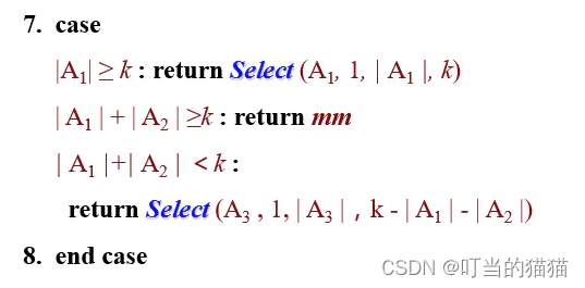
寻找第k小元素 前k小元素 select_k

Oracle recovery tools -- Oracle database recovery tool

论文阅读_中文NLP_LTP
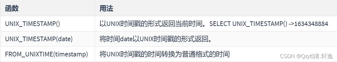
Knowledge points of MySQL (6)
![最大人工岛[如何让一个连通分量的所有节点都记录总节点数?+给连通分量编号]](/img/8b/a60fc36115580f018445e4c2a28a9d.png)
最大人工岛[如何让一个连通分量的所有节点都记录总节点数?+给连通分量编号]

What are the changes in the 2022 PMP Exam?

求解为啥all(())是True, 而any(())是FALSE?
随机推荐
神经网络自我认知模型
EPM相关
mybash
OpenShift常用管理命令杂记
ISPRS2022/云检测:Cloud detection with boundary nets基于边界网的云检测
Neural network self cognition model
Mongodb (quick start) (I)
Operation before or after Teamcenter message registration
数值计算方法 Chapter8. 常微分方程的数值解
Cmake tutorial Step4 (installation and testing)
Vulnerability recurrence - 48. Command injection in airflow DAG (cve-2020-11978)
Sentinel flow guard
Sentinel-流量防卫兵
How awesome is the architecture of "12306"?
Mask wearing detection based on yolov3
深拷贝与浅拷贝【面试题3】
提高應用程序性能的7個DevOps實踐
rsync
证券网上开户安全吗?证券融资利率一般是多少?
读libco保存恢复现场汇编代码