当前位置:网站首页>Study Notes: The Return of Machine Learning
Study Notes: The Return of Machine Learning
2022-08-02 00:07:00 【Menglong is like us】
活动地址:CSDN21天学习挑战赛
1 简介
There are many simple regression problems in life,For example, there is a significant linear relationship between two variables,We can use regression to quantitatively analyze the problem,预测变量.
比如本例子中,We explore the relationship between vehicle speed and brake displacement.
import matplotlib.pyplot as plt
import numpy as np
import pandas as pd
cars=pd.read_csv("../data/cars.csv",usecols=["speed","dist"])
cars[:5]#speed为车速,dist为刹车距离,| 0 | 4 | 2 |
| 1 | 4 | 10 |
| 2 | 7 | 4 |
| 3 | 7 | 22 |
| 4 | 8 | 16 |
查看数据的情况
x=cars["speed"]
y=cars["dist"]
plt.title("fig1.Scatter plot of vehicle speed and braking distance")
plt.scatter(x,y,marker="*",c='red')
From the image we can see that there is roughly some kind of linear relationship between the two variables,Next we quantify it by building a regression model.
2 回归模型
Our purpose is to find the parameters of the following functions

其中x为车速,y为刹车距离.
We need to build a function to measure the difference between the predicted value and the true value,In this way, we can know how the effect of the parameters we finally obtained is.
损失函数为:

n为样本数量, is the real value of a certain braking,
 为预测值.
为预测值.
自然地,我们需要L达到最小值,The regression model obtained in this way is the most accurate,以下有两种方式.
3 两种求解方式
3.1 直接法
The optimal solution can be found directly using the direct method,But it needs to satisfy that the loss function is a convex function,The solution is an analytical solution.
【函数的凹凸性】
Let a function be f(x),There are two points on the image
,弦AB上一点为
.
then stringAB的方程为:
其中
,则
.弦AB的参数方程为:
因为f(x)上任A,Ba little on the stringPThe function value is greater than thenf(x)上的函数值,则有:
 ,弦AB上一点为
 .
.
 ,则
,则 .弦AB的参数方程为:

For the calculation method of parameters, please refer to the blog:最小二乘法
实验部分:
import sympy
#设方程为y=ax+b
#回归系数:比例系数a和偏置值b
a,b=sympy.symbols("a b")
L=0.5*np.sum((y-a*x-b)**2)

#求偏导
f1=sympy.diff(L,b)
f2=sympy.diff(L,a)
print(sympy.diff(L,a))
print(sympy.diff(L,b))

ans=sympy.solve([f1,f2],[b,a])
# Solved{b: -17.5790948905109, a: 3.93240875912409}

alpha=ans[a]
beta=ans[b]
pre=alpha*x+beta
plt.title("Fig2 Fitting results")
plt.scatter(x,y,c="red")
plt.plot(x,pre,c="green")
plt.show()
Draw the resulting straight line:

Then the functional relationship is :

3.2 迭代法
There are limitations to directly optimizing the loss function,If the loss function is a non-convex function, it is difficult to find the optimal solution.Therefore, an iterative method is proposed,Similar to the back-propagation algorithm of the neural network learned earlier,The loss value is minimized by continuously updating the parameters in small increments.所以,The iterative method differs from the direct method in the way the parameters are updated:The former can be obtained by direct calculation,The latter needs to be updated by means of mini-batch gradient descent.
此时损失函数为:

 为批量大小
为批量大小
目标求解:
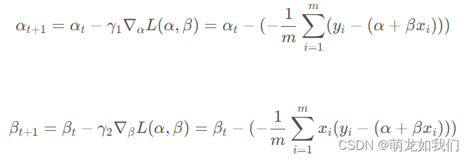
参数更新: 为学习率
为学习率
实验部分:
import  random

#Variable update function
def update_var(pre_alpha,pre_beta,y,x,lr):
    n=len(x)
    diff_alpha=np.sum(-(y-pre_beta*x-pre_alpha))/n
    diff_beta =np.sum(-x*(y-pre_beta*x-pre_alpha))/n
    new_alpha=pre_alpha-lr*diff_alpha
    new_beta=pre_beta-lr*diff_beta

    return (new_alpha,new_beta)

#Implement an iterative process
def iterative_func(y,x,raw_alpha,raw_beta,lr,num,sample_num):
    alpha_list = []
    beta_list = []
    alpha = raw_alpha
    beta = raw_beta
    num_list = list(range(1, len(y)+1))
    for i in range(num):
        alpha_list.append(alpha)
        beta_list.append(beta)
        random.shuffle(num_list)
        index = num_list[:sample_num]
        alpha, beta = update_var(alpha, beta,y[index], x[index], lr)
        print("【{}】Now alpha:{},beta:{}".format(i,alpha,beta))
    return (alpha_list, beta_list)

#随机初始化alpha和beta
raw_alpha=np.random.random()*10
raw_beta =np.random.random()*10
raw_alpha

#设置超参数:学习率lr=0.005  迭代次数num=2000,sample_num=16
lr = 0.005
num = 10000
sample_num = 16
alpha_list, beta_list = iterative_func(y, x, raw_alpha, raw_beta,
lr, num,sample_num)

print("after {} times iteration:alpha: {}, beta:{}".format(num,alpha_list[-1], beta_list[-1]))
after 10000 times iteration:alpha: -17.791370073935074, beta:4.000650060840287
#Persist the data generated by the parameter iteration process
import csv

var_data=zip(alpha_list,beta_list)
with open("../data/20220801_vardata.csv",'w',newline='')as f:
        csv_writer=csv.writer(f)
        csv_writer.writerows(['alpha','beta'])
        csv_writer.writerows(var_data)

plt.subplot(121)
plt.plot(alpha_list)
plt.title("alpha change process")
plt.subplot(122)
plt.plot(beta_list)
plt.title("beta change process")
plt.show()
参考
(44条消息) Machine learning theory and case studies(part2)--回归_GoatGui的博客-CSDN博客
边栏推荐
- Thinkphp 5.0.24变量覆盖漏洞导致RCE分析
- 【Leetcode】1206. Design Skiplist
- Docker实践经验:Docker 上部署 mysql8 主从复制
- recursion: method calls itself
- Leetcode 129求根节点到叶节点数字之和、104二叉树的最大深度、8字符串转换整数(atoi)、82删除排序链表中的重复元素II、204二分查找、94二叉树的中序遍历、144二叉树的前序遍历
- 检查 Oracle 版本的 7 种方法
- Use Jenkins for continuous integration, this knowledge point must be mastered
- Quartus 使用 tcl 文件快速配置管脚
- numpy.where
- Win11内存管理错误怎么办?
猜你喜欢

EasyExcel的简单读取操作

With a monthly salary of 12K, the butterfly changed to a new one and moved forward bravely - she doubled her monthly salary through the career change test~

20220725 Information update

使用Jenkins做持续集成,这个知识点必须要掌握
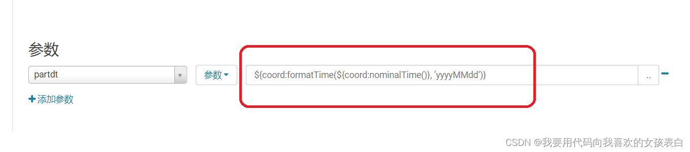
Appears in oozie on CDH's hue, error submitting Coordinator My Schedule

信息系统项目管理师必背核心考点(五十七)知识管理工具

How to get the best power efficiency in Windows 11?
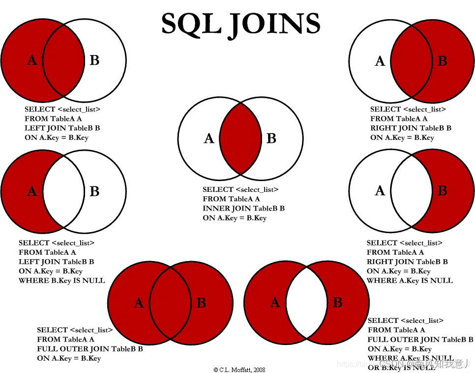
Sql之各种Join
【MySQL系列】MySQL数据库基础

【Leetcode】1206. Design Skiplist
随机推荐
Win10安装DBeaver连接MySQL8、导入和导出数据库详细教程
在MySQL中使用MD5加密【入门体验】
numpy.hstack
分享一份接口测试项目(非常值得练手)
cdh的hue上oozie启动报错,Cannot allocate containers as requested resource is greater than maximum allowed
在linux下MySQL的常用操作命令
Enterprise firewall management, what firewall management tools are there?
如何进行数据库备份
Excel表格数据导入MySQL数据库
Programmer is still short of objects? A new one is enough
async和await用法介绍
Secondary Vocational Network Security Competition B7 Competition Deployment Process
Quartus uses tcl files to quickly configure pins
CDH6的Hue打开出现‘ascii‘ codec can‘t encode characters
几道关于golang并发的面试题
技术分享 | 接口测试中如何使用Json 来进行数据交互 ?
20220725资料更新
获取小猪民宿(短租)数据
C语言七夕来袭!是时候展现专属于程序员的浪漫了!
一个有些意思的项目--文件夹对比工具(一)