[point cloud processing paper crazy reading classic version 10] - pointcnn: revolution on x-transformed points

Abstract

• problem ： CNN Why so successful , That's because convolution operator Be able to take advantage of spatially-local correlation. But point clouds are irregular and disordered , So direct use kernel Convolution of point features will lead to the loss of shape information and the change of point cloud order
• Method ： A simple and general framework is proposed PointCNN, For feature learning of point cloud , Learn from input points $\mathcal{X}$-transformation, It has achieved good results in two aspects ：
  ① The weight of the input feature associated with these points
  ② Map the order of points to a potential and canonical The order of
  stay $\mathcal{X}$-transformation Feature space will also be used convolution operator Multiplication and addition between elements of
• Code ：
  ①https://github.com/yangyanli/PointCNN TensorFlow edition
  ②https://github.com/pyg-team/pytorch_geometric PyTorch edition , This is a library , take PointCNN Encapsulation becomes a function
  ③https://github.com/nicolas-chaulet/torch-points3d Many classic articles are reproduced in a concentrated way

introduction

hypothesis $C$ An unordered set of dimensional input features $\mathbb{F}=\left\{f_a,f_b,f_c,f_d\right\}$ In the figure 1(($i$)-($iv$)) Is the same in all cases , And the size is $4\times C$ Of kernel $\mathbf{K}={\left[k_{\alpha },k_{\beta },k_{\gamma },k_{\delta }\right]}^T$.

In the figure 1($i$) in , The structure of the grid following a given rule , Local $2\times 2$patch The features in can be written with the size $4\times C$ Of ${\left[f_a,f_b,f_c,f_d\right]}^T$, Through and with $\mathbf{K}$ Convolution , obtain $f_i=\mathrm{Conv}\left(\mathbf{K},{\left[f_a,f_b,f_c,f_d\right]}^T\right)$, among $\mathrm{Conv}(\cdot ,\cdot )$ It is a simple multiplication between elements and sum${}^2$ The operation of .

In the figure 1$(ii),(iii)$ and $(iv)$ in , The order of these points is arbitrary . According to the order in the figure , Input feature set $\mathbb{F}$ stay $(ii)$ and $(iii)$ Can be written as ${\left[f_a,f_b,f_c,f_d\right]}^T$, stay $(iv)$ Can be written as ${\left[f_c,f_a,f_b,f_d\right]}^T$. Based on this , If used directly convolution operator, The output characteristics of the three cases are shown in Figure 1 The formula in (1a). We can notice that , In any case $f_{ii}\equiv f_{iii}$ All set up , And in most cases $f_{iii}\ne f_{iv}$ establish . This example shows that the direct use of convolution will lead to the loss of shape information ($f_{ii}\equiv f_{iii}$) And changes in order ($f_{iii}\ne f_{iv}$).

This paper proposes using multi-layer perceptron to learn $K\times K\mathcal{X}$-transformation, Yes $K$ Input point cloud $\left(p_1,p_2,\dots ,p_K\right)$ Coordinate transformation , namely $\mathcal{X}=MLP\left(p_1,p_2,\dots ,p_K\right)$. Our goal is to use this transformation to simultaneously weight and rank the input features , Then convolute the transformed features . The above steps can be called $\mathcal{X}$-Conv, yes PointCNN A foundation in block.$\mathcal{X}$-Conv stay $(ii),(iii)$ and $(iv)$ Can be represented as a graph 1 Chinese formula (1b), among $\mathcal{X}$s It's a $4\times 4$ Matrix , Because in the picture $K=4$. We can notice that , because ${\mathcal{X}}_{ii}$ and ${\mathcal{X}}_{iii}$ It is learned from different shapes , So they can be different , Thus, the corresponding weight is applied to the input characteristics , And achieve $f_{ii}\ne f_{iii}$ The effect of . about ${\mathcal{X}}_{iii}$ and ${\mathcal{X}}_{iv}$, If they can meet after learning ${\mathcal{X}}_{iii}={\mathcal{X}}_{iv}\times \Pi$, among $\Pi$ Yes, it will $(c,a,b,d)$ The order is $(a,b,c,d)$ Sort matrix , Then you can also achieve $f_{iii}\equiv f_{iv}$ The effect of .

Pass diagram 1 We can see from the example analysis in , In the ideal $\mathcal{X}$-transformation Next ,$\mathcal{X}$-Conv Can consider the shape of the point , At the same time, it has sorting invariance . in fact , What we found and learned $\mathcal{X}$-transformation It's far from what we thought , Especially in the aspect of sort invariance . however , be based on $\mathcal{X}$-Conv Of PointCNN The performance of is better than that of the existing methods .

PointCNN

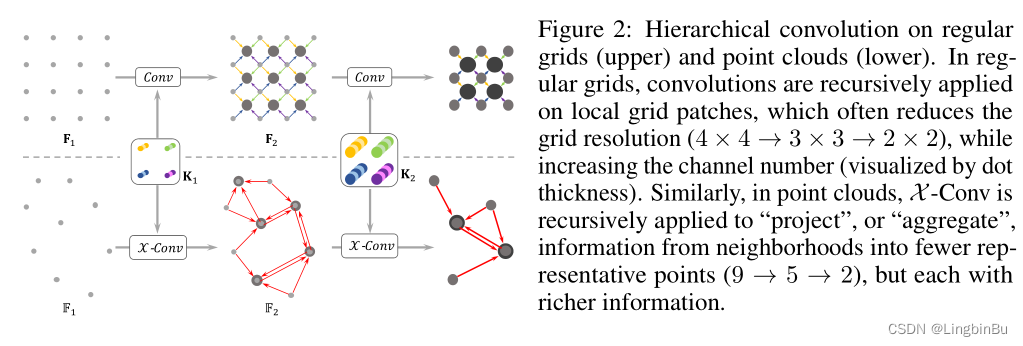
Hierarchical Convolution

Introducing PointCNN Medium hierarchical convolution Before , First, it briefly introduces its application in regular grid , Pictured 2 As shown above . Based on CNN For the grid , The input size is $R_1\times R_1\times C_1$ Characteristic graph ${\mathbf{F}}_1$, among $R_1$ Is the spatial resolution ,$C_1$ The characteristic number of channels is . The size is $K\times K\times C_1\times C_2$ Of kernel and ${\mathbf{F}}_1$ The middle size is $K\times K\times C_1$ Of patches Convolution , Get another size of $R_2\times R_2\times C_2$ Characteristic graph ${\mathbf{F}}_2$. In the figure 2 upper-middle ,$R_1=4,K=2$, $R_2=3$. With the characteristics of ${\mathbf{F}}_1$x comparison ,${\mathbf{F}}_2$ The spatial resolution of is very low ($\left(R_2<R_1\right)$), But with a deeper number of channels ($\left(C_2>C_1\right)$), And have higher-level information .

PointCNN The input is ${\mathbb{F}}_1=\left\{\left(p_{1,i},f_{1,i}\right):i=1,2,\dots ,N_1\right\}$, among $\{p_{1,i}:p_{1,i}\in$${\mathbb{R}}^{\text{Dim }}\}$ It's a set of points , There are also features corresponding to each point $\left\{f_{1,i}:f_{1,i}\in {\mathbb{R}}^{C_1}\right\}$. Based on grid CNN Layered structure , stay ${\mathbb{F}}_1$ On the application $\mathcal{X}$-Conv You can get a higher level of expression ${\mathbb{F}}_2=\left\{\left(p_{2,i},f_{2,i}\right):f_{2,i}\in {\mathbb{R}}^{C_2},i=1,2,\dots ,N_2\right\}$, among $\left\{p_{2,i}\right\}$ yes $\left\{p_{1,i}\right\}$ A group of points of ,${\mathbb{F}}_2$ The spatial resolution ratio of ${\mathbb{F}}_1$ Small ,${\mathbb{F}}_2$ The ratio of the number of channels ${\mathbb{F}}_1$ many , namely $N_2<N_1$, $C_2>C_1$. After the above operation cycle , Features with input points will be “ Projection ” or “ polymerization ” To fewer points , But the characteristic information of each point is richer .

$\left\{p_{2,i}\right\}$ The point in the classification task is through $\left\{p_{1,i}\right\}$ Obtained by random down sampling , In the segmentation task, it is through Farthest Point Sampling(FPS) The algorithm gets , Because the segmentation task requires even point distribution . If there is a better way to choose points , Then the final result will be better , In the future work, we will conduct in-depth research .

$\mathcal{X}$-Conv Operator

$\mathcal{X}$-Conv Operate in a local area of the point cloud , Because the output characteristics should be consistent with the representation point $\left\{p_{2,i}\right\}$ Related to , therefore $\mathcal{X}$-Conv Put them in $\left\{p_{1,i}\right\}$ Neighborhood points in 、 Relevant characteristics as input , To convolute . For a simpler description , remember $p$ by $\left\{p_{2,i}\right\}$ Points in ,$p$ Is characterized by $f$,$p$ stay $\left\{p_{1,i}\right\}$ The adjacent points of are $\mathbb{N}$. therefore , For a particular point $p$ for ,$\mathcal{X}$-Conv The input is $\mathbb{S}=\left\{\left(p_i,f_i\right):p_i\in \mathbb{N}\right\}$.$\mathbb{S}$ Is an unordered set . Without losing generality ,$\mathbb{S}$ It can be written. $K\times Dim$ Matrix $\mathbf{P}={\left(p_1,p_2,\dots ,p_K\right)}^T$ and $K\times C_1$ Matrix $\mathbf{F}={\left(f_1,f_2,\dots ,f_K\right)}^T$,$\mathbf{K}$ It means to train kernel. With these inputs , You can calculate $p$ The output characteristics of ：
$${\mathbf{F}}_p=\mathcal{X}-\mathrm{Conv}(\mathbf{K},p,\mathbf{P},\mathbf{F})=\mathrm{Conv}\left(\mathbf{K},\mathrm{MLP}(\mathbf{P}-p)\times \left[ML{P}_{\delta }(\mathbf{P}-p),\mathbf{F}\right]\right),$$
among $ML{P}_{\delta }(\cdot )$ It is a multi-layer perceptron acting on a single point , stay $\mathcal{X}$-Conv All operations ,$\mathrm{Conv}(\cdot ,\cdot ),\mathrm{MLP}(\cdot )$, Matrix multiplication $(\cdot )\times (\cdot )$ and $ML{P}_{\delta }(\cdot )$ It's all derivable , that $\mathcal{X}$-Conv It's also derivable , So it can be used in other back propagation neural networks .

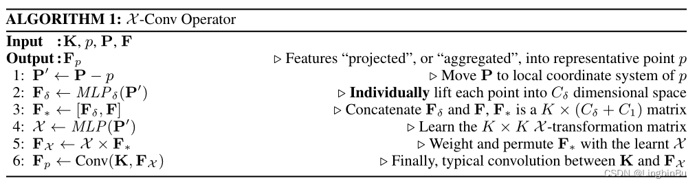
Algorithm 1 No 4-6 Line mainly expresses the equation 1b($\mathcal{X}$-transformation).

Algorithm 1 No 1-3 In line , Normalize the neighborhood points to points $p$ On the relative position of , So as to obtain local features . When outputting features , Neighborhood points and corresponding features need to be determined together , But the dimension and representation of local coordinates are different from the corresponding features . To solve this problem , First, raise the coordinates to a higher dimension and a more abstract representation ( Such as algorithm 1 Of the 2 Line ), Then it is spliced with the corresponding features ( Algorithm 1 Of the 3 That's ok ), For later processing ( chart 3 c).

adopt point-wise $ML{P}_{\delta }(\cdot )$ Map coordinates to features , This is related to PointNet The methods used in are similar , The difference is that symmetric functions are not used for processing . This passage $\mathcal{X}$-transformation Weight and sort coordinates and features , This $\mathcal{X}$-transformation It is learned by all adjacent points . The final $\mathcal{X}$ Depends on the order of points , This is expected , because $\mathcal{X}$ The pairs should be arranged according to the input points ${\mathbf{F}}_{\ast }$ Sort , Therefore, you must know the specific input order . For input point clouds without any additional features , namely $\mathbf{F}$ It's empty , first $\mathcal{X}$-Conv Layers only use ${\mathbf{F}}_{\delta }$. therefore ,PointCNN Point clouds with or without additional features can be handled in a robust general way .
$\mathcal{X}$

PointCNN Architectures

Conv layers in grid-based CNNs and $\mathcal{X}$-Conv layers in PointCNN There are two differences ：

1. The methods of local feature extraction are different ($K\times K$ patches vs. Indicates $K$ Adjacent points )
2. There are different ways to learn from local areas (Conv vs. $\mathcal{X}$-Conv)

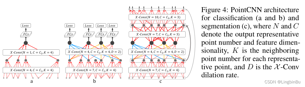
chart 4(a) Describes one with two $\mathcal{X}$-Conv Layer of PointCNN structure , Will enter a point ( With or without features ) Gradually become few representation points , But these points have rich characteristics . In the second $\mathcal{X}$-Conv After the layer , There is only one representation point left , This is the representation point from which the information of all points in the previous layers is aggregated . stay PointCNN in , The perception domain of each representation point can be defined as a proportion $K/N$, among $K$ Is the number of adjacent points ,$N$ Is the number of points on the previous floor . such , The last point can “ notice ” Points of all previous layers , Therefore, the proportion of its perception domain is 1.0—— It has a global view of the entire shape , And its features are also very informative for the semantic understanding of shapes . At the end of the $\mathcal{X}$-Conv Add a full connection layer behind the layer , Then we can train the network with a loss function .

We noticed that the number of points is above $\mathcal{X}$-Conv The layer drops quickly ( chart 4a), It makes the simple network unable to carry out comprehensive training . To solve this problem , A method with dense connections is proposed PointCNN Model , Pictured 4b Shown . stay $\mathcal{X}$-Conv More representation points are reserved in the layer . however , Our goal is to keep the depth of the network unchanged , While maintaining the growth rate of the perception domain , Only such a deep expression point can “ notice ” A larger area of the whole shape . therefore , stay PointCNN From grid-based CNNs Borrowed from dilated convolution thought . No longer in a fixed $K$ Adjacent points as input , But randomly from $K\times D$ Randomly sampled from adjacent points $K$ Input points , among $D$ yes dilation rate. under these circumstances , Without increasing the sum of the actual number of adjacent points kernel In case of size , The proportion of perception domain ranges from $K/N$ Growth to $(K\times D)/N$.

And graph 4a comparison , chart 4b Last of all $\mathcal{X}$-Conv Layer. 4 All points are ok “ notice ” Entire shape , Therefore, they are suitable for prediction . In the test phase ,softmax Previously, multiple prediction results can be averaged , Make the prediction result more stable .

For split tasks , You need to output the original resolution points , This can be done by constructing Conv-DeConv Structure implementation , among DeConv Part is the process of spreading global information to higher resolution prediction , See the picture 4c. It is worth noting that ,PointCNN Segment the network “Conv” and “DecConv” It's all the same $\mathcal{X}$-Conv operation .“Conv” and “DeConv” The only difference between them is that the output of the latter has more points , Fewer channels .

Use in front of the last full connection layer dropout Reduce over fitting , Also used. subvolume supervision Further reduce over fitting . At the end of the $\mathcal{X}$-Conv Layer , The proportion of perception domain is set to be less than 1 Number of numbers , So that only part of the information is observed . In the process of training , The network is required to learn more difficult from some information , In this way, it will perform better in the test . under these circumstances , It is important to represent the global coordinates of points , So by $ML{P}_g(\cdot )$ Promote the global coordinates to the feature space ${\mathbb{R}}^{C_g}$, And spliced to $\mathcal{X}$-Conv in , For further processing through subsequent layers .

Data augmentation

To improve generalization , Random sampling of input points and shuffle, such batch And batch The set and order of adjacent points will be different . In order to train a quantity of $N$ As input , choice $\mathcal{N}(N,(N/8{)}^2)$ Points for training , among $\mathcal{N}$ Represents Gaussian distribution , This is good for PointCNN Training is crucial .

experiment

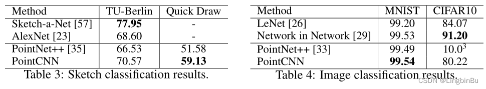
Classification

Segmentation

Ablation Experiments

Visualizations

Optimizer, model size, memory usage and timing

Conclusion

• How to understand and propose the effectiveness of the network is still a big problem
• take PointCNN And imageCNN It is also a very interesting field to combine processing pairs of point clouds and images