Matlab tips (23) matrix analysis -- simulated annealing

Preface

MATLAB Learning about image processing is very friendly , You can start from scratch , There are many encapsulated functions that can be called directly for basic image processing , This series of articles is mainly to introduce some of you in MATLAB Some concept functions are commonly used in routine demonstration ！

Simulated annealing algorithm （Simulate Anneal Arithmetic,SAA） It's a general probability algorithm , It is used to find the optimal solution of a proposition in a large search space . Simulated annealing is S.Kirkpatrick, C.D.Gelatt and M.P.Vecchi stay 1983 Invented in . and V.Černý stay 1985 The algorithm was also independently invented in . Simulated annealing algorithm is to solve TSP One of the effective ways to solve the problem .

One . Simulated annealing basis

Simulated annealing comes from the term annealing in metallurgy . Annealing is the process of heating a material and then cooling it at a specific rate , The purpose is to increase the volume of grains , And reduce defects in the lattice . The atoms in the material will stay at the position where the internal energy has a local minimum , Heating increases energy , The atom will leave its original position , And random moves in other places . Annealing cooling is slower , It makes it possible for atoms to find positions with lower internal energy than before .

The principle of simulated annealing is similar to that of metal annealing ： Apply the theory of thermodynamics to statistics , Think of searching every point in space as a molecule in the air ; Molecular energy , It's the kinetic energy of itself ; And search every point in space , It's also like air molecules with “ energy ”, To show the suitability of the point to the proposition . The algorithm starts by searching for an arbitrary point in space ： Choose one at each step “ neighbor ”, And then calculate how to get from the existing position to “ neighbor ” Probability .

Simulated annealing algorithm can be decomposed into solution space 、 Objective function and initial solution .

The basic idea of simulated annealing :

(1) initialization ： initial temperature T( Big enough ), The initial solution state S( It's the starting point of algorithm iteration ), Every T The number of iterations of the value L;

(2) Yes k=1,……,L Do the first (3) To 6 Step ;

(3) New solutions S′;

(4) Calculate increment Δt′=C(S′)-C(S), among C(S) Is the evaluation function ;

(5) if Δt′<0 received S′ As a new current solution , Otherwise, with probability exp(-Δt′/T) To take over S′ As a new current solution ;

(6) If the termination condition is satisfied, the current solution is output as the optimal solution , End procedure . The termination condition is usually taken as terminating the algorithm when several new solutions are not accepted ;

(7) T Gradually reduce , And T->0, And then turn to 2 Step ;

The generation and acceptance of the new solution of simulated annealing algorithm can be divided into the following four steps ：

First step ： A generating function generates a new solution in the solution space from the current solution ; For the convenience of subsequent calculation and acceptance , Reduce algorithm time , In general, the method of generating a new solution by simply transforming the current solution is chosen , For example, replace all or part of the elements constituting the previous solution 、 Swap, etc , Note that the transformation method of generating the new solution determines the neighborhood structure of the current new solution , Therefore, it has a certain influence on the selection of cooling schedule .

The second step ： Calculate the difference between the objective function corresponding to the new solution . Because the objective function difference is only generated by the transformation part , So it's better to calculate the difference of objective function by increment . It turns out that , For most applications , This is the fastest way to calculate the difference of the objective function .

The third step ： Judge whether the new solution is accepted , The basis of judgment is an acceptance criterion , The most common acceptance criteria are Metropolis Rules : if Δt′<0 received S′ As a new current solution S, Otherwise, with probability exp(-Δt′/T) Accept S′ As a new current solution S.

Step four ： When the new solution is determined to be accepted , Replace the current solution with a new one , This only needs to realize the transformation part of the current solution corresponding to the new solution , At the same time, the objective function value can be modified . here , The current solution implements an iteration . On this basis, we can start the next round of tests . And when the new solution is judged to be abandoned , On the basis of the original current solution, the next round of test is continued .

The example encountered when searching for data , Here to share ,MATLAB Version is MATLAB2015b.

Two . MATLAB Fake one

%%%%%%%%%%%%%%%%%%%%%%%%%%%%%%%%%%%%%%%%%%%%%%%%%%%%
% function ： matrix analysis -- Simulated annealing 
% Environmental Science ：Win7,Matlab2015b
%Modi: C.S
% Time ：2022-06-27
%%%%%%%%%%%%%%%%%%%%%%%%%%%%%%%%%%%%%%%%%%%%%%%%%%%%


%% I.  Clear environment variables 
clear all
clc

tic
%% II.  Unary function optimization 
x = 1:0.01:2;
y = sin(10*pi*x) ./ x;
figure
plot(x,y,'linewidth',1.5)
ylim([-1.5, 1.5])
xlabel('x')
ylabel('y')
title('y = sin(10*pi*x) / x')
hold on

%%
% 1.  Mark the maximum point 
[maxVal,maxIndex] = max(y);
plot(x(maxIndex), maxVal, 'r*','linewidth',2)
text(x(maxIndex), maxVal, {
    [' X: ' num2str(x(maxIndex))];[' Y: ' num2str(maxVal)]})
hold on

%%
% 2.  Mark the minimum point 
[minVal,minIndex] = min(y);
plot(x(minIndex), minVal, 'ks','linewidth',2)
text(x(minIndex), minVal, {
    [' X: ' num2str(x(minIndex))];[' Y: ' num2str(minVal)]})

%% III.  Bivariate function optimization 
[x,y] = meshgrid(-5:0.1:5,-5:0.1:5);
z = x.^2 + y.^2 - 10*cos(2*pi*x) - 10*cos(2*pi*y) + 20;
figure
mesh(x,y,z)
hold on
xlabel('x')
ylabel('y')
zlabel('z')
title('z =  x^2 + y^2 - 10*cos(2*pi*x) - 10*cos(2*pi*y) + 20')

%%
% 1.  Mark the maximum point 
maxVal = max(z(:));
[maxIndexX,maxIndexY] = find(z == maxVal);
for i = 1:length(maxIndexX)
    plot3(x(maxIndexX(i),maxIndexY(i)),y(maxIndexX(i),maxIndexY(i)), maxVal, 'r*','linewidth',2)
     text(x(maxIndexX(i),maxIndexY(i)),y(maxIndexX(i),maxIndexY(i)), maxVal, {
    [' X: ' num2str(x(maxIndexX(i),maxIndexY(i)))];[' Y: ' num2str(y(maxIndexX(i),maxIndexY(i)))];[' Z: ' num2str(maxVal)]})
    hold on
end
toc

Click on “ function ”, The results are as follows ：

3、 ... and . MATLAB Simulation II

%%%%%%%%%%%%%%%%%%%%%%%%%%%%%%%%%%%%%%%%%%%%%%%%%%%%
% function ： matrix analysis -- Simulated annealing 
% Environmental Science ：Win7,Matlab2015b
%Modi: C.S
% Time ：2022-06-27
%%%%%%%%%%%%%%%%%%%%%%%%%%%%%%%%%%%%%%%%%%%%%%%%%%%%

%% I.  Clear environment variables 
clear all
clc

tic
%% II.  Import city location data 
X = [16.4700   96.1000
     16.4700   94.4400
     20.0900   92.5400
     22.3900   93.3700
     25.2300   97.2400
     22.0000   96.0500
     20.4700   97.0200
     17.2000   96.2900
     16.3000   97.3800
     14.0500   98.1200
     16.5300   97.3800
     21.5200   95.5900
     19.4100   97.1300
     20.0900   92.5500];

%% III.  Calculate distance matrix 
D = Distance(X);  % Calculate distance matrix 
N = size(D,1);    % Number of cities 

%% IV.  Initialize parameters 
T0 = 1e10;   %  initial temperature 
Tend = 1e-30;  %  Termination temperature 
L = 2;    %  Number of iterations at each temperature 
q = 0.9;    % Cooling rate 
Time = ceil(double(solve([num2str(T0) '*(0.9)^x = ',num2str(Tend)])));  %  Calculate the number of iterations 
% Time = 132;
count = 0;        % Iteration count 
Obj = zeros(Time,1);         % Initialization of target value matrix 
track = zeros(Time,N);       % The optimal route matrix of each generation is initialized 

%% V.  Randomly generate an initial route 
S1 = randperm(N);
DrawPath(S1,X)
disp(' A random value in the initial population :')
OutputPath(S1);
Rlength = PathLength(D,S1);
disp([' Total distance ：',num2str(Rlength)]);

%% VI.  Iterative optimization 
while T0 > Tend
    count = count + 1;     % Update iterations 
    temp = zeros(L,N+1);
    %%
    % 1.  New solutions 
    S2 = NewAnswer(S1);
    %%
    % 2. Metropolis The law determines whether to accept the new solution 
    [S1,R] = Metropolis(S1,S2,D,T0);  %Metropolis  Sampling algorithm 
    %%
    % 3.  Record the best route for each iteration 
    if count == 1 || R < Obj(count-1)
        Obj(count) = R;           % If the optimal distance at the current temperature is less than the previous distance, record the current distance 
    else
        Obj(count) = Obj(count-1);% If the optimal distance at the current temperature is greater than the previous distance, record the previous distance 
    end
    track(count,:) = S1;
    T0 = q * T0;     % cool 
end

%% VII.  Iteration diagram of optimization process 
figure
plot(1:count,Obj)
xlabel(' The number of iterations ')
ylabel(' distance ')
title(' The optimization process ')

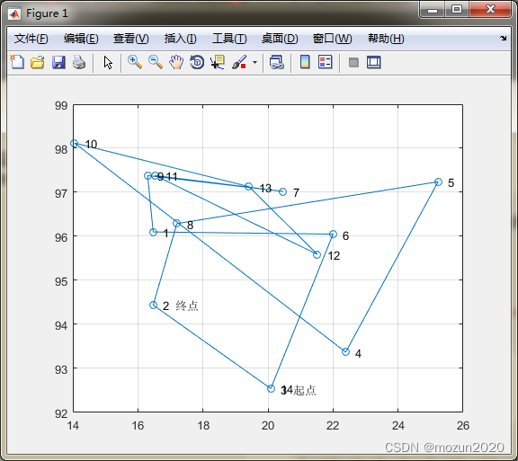
%% VIII.  Draw the optimal path map 
DrawPath(track(end,:),X)

%% IX.  The route and total distance of the output optimal solution 
disp(' Optimal solution :')
S = track(end,:);
p = OutputPath(S);
disp([' Total distance ：',num2str(PathLength(D,S))]);
toc

Click on “ function ”, The results are as follows ：

 A random value in the initial population :
3—>14—>6—>1—>9—>7—>11—>12—>13—>10—>4—>5—>8—>2—>3
 Total distance ：60.8861
 Optimal solution :
11—>9—>10—>2—>14—>3—>4—>5—>6—>12—>7—>13—>8—>1—>11
 Total distance ：29.6889
 Time has passed  1.465166  second .

Four . Summary

Simulated annealing algorithm is widely used , It can solve the maximum cut problem with high efficiency (Max Cut Problem)、0-1 knapsack problem (Zero One Knapsack Problem)、 Graph coloring problem (Graph Colouring Problem)、 Scheduling problem (Scheduling Problem) wait . This example , It may be used later , Take a note . Learn one every day MATLAB Little knowledge , Let's learn and make progress together ！