当前位置:网站首页>[data mining] visual pattern mining: hog feature + cosine similarity /k-means clustering
[data mining] visual pattern mining: hog feature + cosine similarity /k-means clustering
2022-07-07 15:07:00 【zstar-_】
1. An overview of the experiment
This experiment uses VOC2012 Data sets , First, randomly sample image blocks from the image , And then use it Hog Methods extract image block features , Finally, cosine similarity and k-means Clustering two methods to mine visual patterns .
2. Data set description
This experiment uses VOC2012 Data sets .VOC2012 Data sets are often used for target detection 、 Image segmentation 、 Network comparison experiment and model effect evaluation . For image segmentation tasks ,VOC2012 The training validation set of contains 2007-2011 All corresponding images of the year , contains 2913 Pictures and 6929 Goals , The test set contains only 2008-2011 year .
Because this data set is mostly used in tasks such as target detection , So in this experiment , Use only... In this dataset 8 Class data .
Dataset download link :
http://host.robots.ox.ac.uk/pascal/VOC/voc2012/index.html
3. Introduction to algorithm model
3.1 Hog feature extraction
Direction gradient histogram (Histogram of Oriented Gradient, HOG) Feature is a kind of feature descriptor used for object detection in computer vision and image processing . It constructs the feature by calculating and counting the histogram of gradient direction in the local region of the image , Its main steps are as follows :
- Graying
Grayscale the picture , Filter out irrelevant color information . - Standardization of color space
use Gamma The input image is normalized in color space by correction method , You can adjust the contrast of the image , Reduce the impact of local shadow and light changes in the image , At the same time, it can suppress the interference of noise . - Gradient calculation
Calculate the gradient of each pixel in the image ( Including size and direction ), It can capture contour information , At the same time, further weaken the interference of light . - Cell Divide
Divide the image into small cells, With 8x8 The size of Cell For example , As shown in the figure :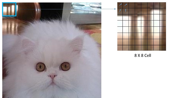
- Count each one cell The gradient histogram of
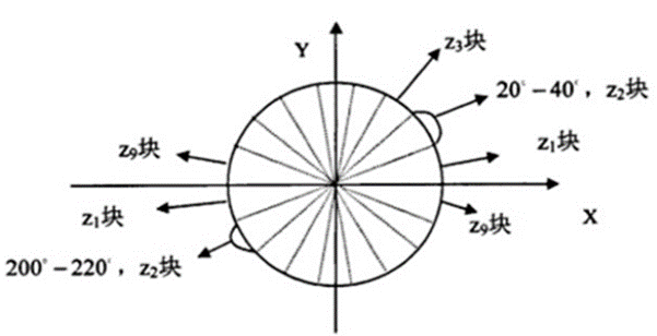
As shown in the figure , take 360° Divide into 18 Share , Each angle is 20°. meanwhile , Regardless of direction , That is, a total of 9 Angle category , Count the frequency of each category . - Will each several cell Form a block
With 2x2 The size of block For example , As shown in the figure :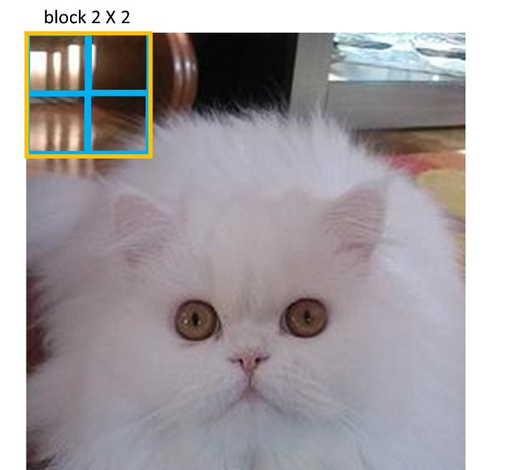
The blue box in the figure indicates a cell, The yellow box indicates a block, take 2x2 individual cell Make up a block, At the same time in each block Normalize the gradient histogram . There are four main normalization methods :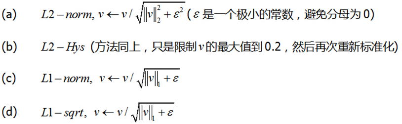
The original paper states L2-Hys It's the best way [1], So in this experiment , The normalization method also uses L2-Hys. - Move block
Each one block With cell Move horizontally and vertically for spacing , Finally, all feature vectors are concatenated to get the Hog features .
3.2 Cosine similarity
Get the of each image block Hog After feature , The classification is carried out by calculating the cosine similarity of each image block feature vector , The calculation formula of cosine similarity is as follows :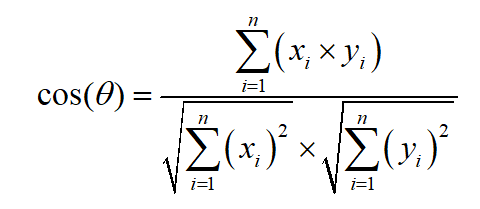
3.3 K-means clustering
Get the of each image block Hog After features , You can also use K-means Clustering to mine visual patterns .K-means The process of clustering is shown in the figure :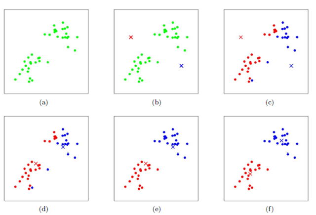
First, two points are initialized randomly as clustering centers , Calculate the distance from each point to the cluster center , And cluster to the nearest cluster . after , Calculate the average coordinates of all points in each cluster , And take this average as a new clustering center ; Repeat these two steps , Until the cluster center of each class no longer changes , Complete clustering .
4. Frequency and discriminant evaluation indicators
4.1 Frequency evaluation index
If a pattern appears many times in a positive image , It is called frequent . In this experiment , The evaluation index of frequency refers to Wang Qiannan et al [2] The evaluation criteria of , Define the frequency formula as follows :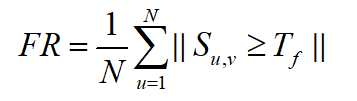
In style ,N Represents the total number of samples of a certain type , S u , v S_{u,v} Su,v Represents the sample in this class u And the sample v Cosine similarity of , T f T_f Tf Represents the threshold .
4.2 Discriminant evaluation index
If a mode value appears in a positive image , Not in negative images , It is called discriminative . In this experiment , The average classification accuracy of visual patterns is used to define discrimination , The formula is as follows :
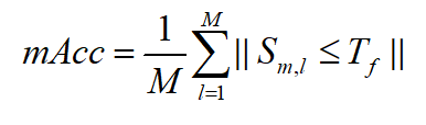
In style ,M Represents the total number of sample categories , S m , l S_{m,l} Sm,l Represents the average value of the visual pattern of the sample in the class m And the sample v Cosine similarity of , T f T_f Tf Represents the threshold .
5. The experimental steps
5.1 Data set classification
This experiment adopts VOC2012 Data sets , Pictures are not classified by category . Therefore, first of all, according to the category , Divide the pictures containing this category . A total of 7 Categories :“ vehicle 、 Horse 、 cat 、 Dog 、 bird 、 sheep 、 cattle ”.
The core code for executing the partition is as follows :
def get_my_classes(Annotations_path, image_path, save_img_path, classes):
    xml_path = os.listdir(Annotations_path)
    for i in classes:
        if not os.path.exists(save_img_path+"/"+i):
            os.mkdir(save_img_path+i)
    for xmls in xml_path:
        print(Annotations_path+"/"+xmls)
        in_file = open(os.path.join(Annotations_path, xmls))
        print(in_file)
        tree = ET.parse(in_file)
        root = tree.getroot()
        if len(set(root.iter('object'))) != 1:
            continue
        for obj in root.iter('object'):
            cls_name = obj.find('name').text
            print(cls_name)
        try:
            shutil.copy(image_path+"/"+xmls[:-3]+"jpg", save_img_path+"/"+cls_name+"/"+xmls[:-3]+"jpg")
        except:
            continue
The result of code execution is as follows :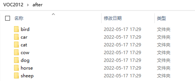
5.2 Image block sampling
To sample image blocks , In this experiment, the method of random clipping is selected . Take the center point of each image as the benchmark , stay [- Picture length and width /6, Picture length and width /6] The center point is offset within the limited range of , So as to obtain the sampled image block , The sampling process is shown in the figure :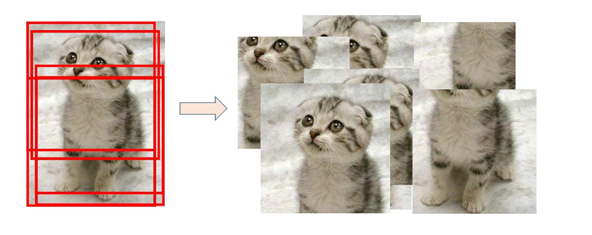
For each image , Total random sampling 10 Sample blocks , The core code is as follows :
for each_image in os.listdir(IMAGE_INPUT_PATH):
  #  Full path of each image
  image_input_fullname = IMAGE_INPUT_PATH + "/" + each_image
  #  utilize PIL Library opens every image
  img = Image.open(image_input_fullname)
  #  Define crop picture left 、 On 、 Right 、 Pixel coordinates under
  x_max = img.size[0]
  y_max = img.size[1]
  mid_point_x = int(x_max/2)
  mid_point_y = int(y_max/2)
  for i in range(0, 10):
      #  The center point is randomly offset
      crop_x = mid_point_x + \
          random.randint(int(-mid_point_x/3), int(mid_point_x/3))
      crop_y = mid_point_y + \
          random.randint(int(-mid_point_y/3), int(mid_point_y/3))
      dis_x = x_max-crop_x
      dis_y = y_max-crop_y
      dis_min = min(dis_x, dis_y, crop_x, crop_y)  #  Get the range of change
      down = crop_y + dis_min
      up = crop_y - dis_min
      right = crop_x + dis_min
      left = crop_x - dis_min
      BOX_LEFT, BOX_UP, BOX_RIGHT, BOX_DOWN = left, up, right, down
      #  Return a rectangular area from the original image , Area is a 4 Tuples define the upper left and lower right pixel coordinates
      box = (BOX_LEFT, BOX_UP, BOX_RIGHT, BOX_DOWN)
      #  Conduct roi tailoring
      roi_area = img.crop(box)
      #  The path of each image after clipping + name
      image_output_fullname = IMAGE_OUTPUT_PATH + \
          "/" + str(i) + "_" + each_image
      #  Store the cropped image
      roi_area.save(image_output_fullname)
5.3 Hog feature extraction
For each image block , Adjust its size to 256x256, And normalize it , Extract it Hog features , The core code is as follows :
#  Image preprocessing
def preprocessing(src):
    gray = cv2.cvtColor(src, cv2.COLOR_BGR2GRAY)  #  Convert image to grayscale image
    img = cv2.resize(gray, (256, 256))  #  Size adjustment g
    img = img/255.0    #  Data normalization
    return img
#  extract hog features
def extract_hog_features(X):
    image_descriptors = []
    for i in range(len(X)):
        '''  Parameter interpretation : orientations: Direction number  pixels_per_cell: Cell size  cells_per_block: Block size  block_norm: Optional block normalization method L2-Hys(L2 norm ) '''
        fd, _ = hog(X[i], orientations=9, pixels_per_cell=(
            16, 16), cells_per_block=(16, 16), block_norm='L2-Hys')
        image_descriptors.append(fd)  #  Stitching all the images hog features
    return image_descriptors        #  All images of the training part are returned hog features
there cell The size is (16,16),block The size is (16,16).
5.4 Mining through cosine similarity
According to the Hog features , Use the criteria of frequency and discrimination to calculate , The core code is as follows :
threshold = 0.6
group1 = []
group2 = []
group1.append(X_features[0])
for i in range(1, len(X_features)):
   res = cosine_similarity(X_features[0].reshape(1, -1), X_features[i].reshape(1, -1))
   if res > threshold:
       group1.append(X_features[i])
   else:
       group2.append(X_features[i])
According to the literature [2] Experience , The thresholds here are 0.6,0.7,0.8, The experimental results are shown in the next section .
5.5 adopt k-means Clustering method for mining
In this experiment , Another way is also adopted, that is k-means Clustering is a way to mine visual patterns , The core code is as follows :
cluster = KMeans(n_clusters=2, random_state=0)
y = cluster.fit_predict(X_features)
colors = ['blue', 'red']
plt.figure()
for i in range(len(y)):
    plt.scatter(X_features[i][0], X_features[i][1], color=colors[y[i]])
plt.title(" The first two dimensions are clustered to represent ")
plt.savefig("cluster.png")
plt.show()
With “ sheep ” As a frequent mining category , The first two dimensions of the mined positive and negative samples are visualized as follows :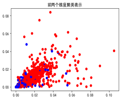
After extracting frequent visual patterns , Mining for discrimination , The method of cosine similarity is still used , The results are shown in the next section .
6. experimental result
The category selected for this experiment is “ sheep ”(sheep), Two methods and different cosine similarity thresholds are used , The numerical results are shown in the table below :
| threshold | Frequency |
|---|---|
| 0.6 | 0.623 |
| 0.7 | 0.863 |
| 0.8 | 0.999 |
You can find , As the threshold increases , The more frequent the mined visual patterns are .
| threshold | car | horse | cat | dog | bird | cow | Average discriminant |
|---|---|---|---|---|---|---|---|
| 0.6 | 0.887 | 0.291 | 0.315 | 0.258 | 0.489 | 0.144 | 0.397 |
| 0.7 | 0.957 | 0.513 | 0.64 | 0.567 | 0.708 | 0.382 | 0.628 |
| 0.8 | 0.988 | 0.791 | 0.914 | 0.841 | 0.873 | 0.716 | 0.854 |
Similar , As the threshold increases , The more discriminative the mined visual patterns are , When the threshold value is 0.8 when , The highest average discriminant is 0.854.
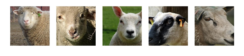
The visual patterns mined by this method , The visualization part is as follows :
In this experiment K-means Mining visual patterns by clustering , The obtained frequency value is 0.707, For discriminative calculation , The method of cosine similarity is still used , The results are shown in the table below :
| threshold | car | horse | cat | dog | bird | cow | Average discriminant |
|---|---|---|---|---|---|---|---|
| 0.6 | 0.883 | 0.26 | 0.299 | 0.242 | 0.493 | 0.146 | 0.387 |
| 0.7 | 0.956 | 0.503 | 0.632 | 0.569 | 0.713 | 0.391 | 0.627 |
| 0.8 | 0.987 | 0.793 | 0.91 | 0.843 | 0.879 | 0.724 | 0.856 |
Similar to the previous method , As the threshold increases , The more discriminative the mined visual patterns are , When the threshold value is 0.8 when , The highest average discriminant is 0.856.
The visual patterns mined by this method , The visualization part is as follows :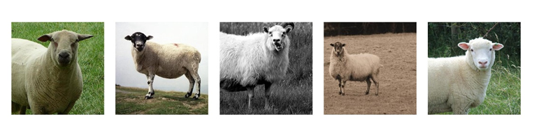
The figure is visible , Although the visual patterns mined by the two methods have little difference in value , But the visualization results are different . The visual patterns mined by cosine similarity method are more about the facial features of sheep , and K-means The visual patterns mined by clustering are more about the physical characteristics of sheep .
7. Summary of the experiment
This experiment , Using the traditional Hog Feature extraction method , And use cosine similarity and K-means Mining visual patterns by clustering . Through this experiment , It can be found that there may be more than one visual mode of a certain kind of picture , In this experiment , Multiple visual modes are not considered . In this case , Adopt density based clustering [2] May be more suitable .
Besides , For visual pattern mining , Such as Hog、Sift And other traditional feature extraction methods , The representation ability is not strong , No abstract ability . Use similar CNN Neural network is a more mainstream and effective way at present .
reference
[1] N Dalal, B Triggs. Histograms of Oriented Gradients for Human Detection [J]. IEEE Computer Society Conference on Computer Vision & Pattern Recognition, 2005, 1(12): 886-893.
[2] Wang Qiannan . Research on visual pattern mining algorithm based on deep learning [D]. Xi'an University of Electronic Science and Technology ,2021.DOI:10.27389/d.cnki.gxadu.2021.002631.
Complete source code
Experimental report + Source code :
link :https://pan.baidu.com/s/131RbDp_LNGhmEaFREvgFdA?pwd=8888
Extraction code :8888
边栏推荐
- Electronic remote error
- Five pain points for big companies to open source
- Discussion on CPU and chiplet Technology
- 【深度学习】图像超分实验:SRCNN/FSRCNN
- JSON解析实例(Qt含源码)
- What is cloud primordial? This time, I can finally understand!
- Ctfshow, information collection: web1
- 最安全的证券交易app都有哪些
- Niuke real problem programming - Day12
- [server data recovery] data recovery case of raid failure of a Dell server
猜你喜欢

Deformable convolutional dense network for enhancing compressed video quality
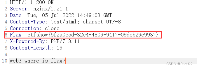
CTFshow,信息搜集:web3
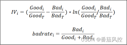
知否|两大风控最重要指标与客群好坏的关系分析

Spatiotemporal deformable convolution for compressed video quality enhancement (STDF)
![leetcode:648. Word replacement [dictionary tree board + find the shortest matching prefix among several prefixes]](/img/3e/cdde4b436821af8700eb65d35e8f59.png)
leetcode:648. Word replacement [dictionary tree board + find the shortest matching prefix among several prefixes]
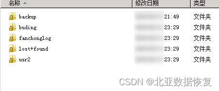
【服务器数据恢复】某品牌StorageWorks服务器raid数据恢复案例
Niuke real problem programming - Day12
[server data recovery] a case of RAID data recovery of a brand StorageWorks server

Qu'est - ce qu'une violation de données
What is data leakage
随机推荐
Today's sleep quality record 78 points
Yyds dry goods inventory # solve the real problem of famous enterprises: cross line
什么是pv和uv? pv、uv
8大模块、40个思维模型,打破思维桎梏,满足你工作不同阶段、场景的思维需求,赶紧收藏慢慢学
A laravel background management expansion package you can't miss - Voyager
What is the process of ⼀ objects from loading into JVM to being cleared by GC?
leetcode:648. Word replacement [dictionary tree board + find the shortest matching prefix among several prefixes]
WebRTC 音频抗弱网技术(上)
Novel Slot Detection: A Benchmark for Discovering Unknown Slot Types in the Dialogue System
什么是数据泄露
Change win10 Screensaver
#yyds干货盘点# 解决名企真题:交叉线
Ctfshow, information collection: web10
15、文本编辑工具VIM使用
Ctfshow, information collection: web7
JSON parsing instance (QT including source code)
13 ux/ui/ue best creative inspiration websites in 2022
CTFshow,信息搜集:web12
Niuke real problem programming - Day17
Apache多个组件漏洞公开(CVE-2022-32533/CVE-2022-33980/CVE-2021-37839)