Matlab tips (24) RBF, GRNN, PNN neural network

Preface

MATLAB Learning about image processing is very friendly , You can start from scratch , There are many encapsulated functions that can be called directly for basic image processing , This series of articles is mainly to introduce some of you in MATLAB Some concept functions are commonly used in routine demonstration ！

RBF The neural network is divided into three layers , The first layer is the input layer, that is Input Layer, It is composed of signal source nodes ; The second layer is the hidden layer, that is, the yellow ball in the middle of the figure , And the radial basis function of the radial basis function is a non symmetric radial function , The function is a local response function . Because it's a local corresponding function , Therefore, the number of neurons in the hidden layer should be set according to the specific problem ; The third layer is the output layer , Is the response to the input pattern , The output layer adjusts the linear weight , The linear optimization strategy is adopted , So learning speed is faster .

GRNN Generalized regression neural network is a kind of radial basis function neural network ,GRNN It has strong nonlinear mapping ability and learning speed , Than RBF Have a stronger advantage , Finally, the network converges to the optimal regression with more sample size , When the sample data is small , The prediction effect is very good , It can also handle unstable data . although GRNN It seems that there is no radial basis function , But in fact, in classification and fitting , Especially when the data accuracy is relatively poor, it has great advantages .

PNN（Product-based Neural Network） Is in 2016 Proposed in to calculate CTR Deep neural network model of the problem ,PNN The network structure of traditional FNN（Feedforward Neural Network） The network structure has been optimized , Make it more suitable for dealing with CTR problem .

Radial basis function neurons and linear neurons can establish Generalized Regression Neural Networks GRNN, It is RBF A variation of the network , Often used for function approximation . In some ways RBF The network has more advantages . Radial basis function neurons and competitive neurons can also form Probabilistic Neural Networks PNN.PNN It's also RBF A variation of , Simple structure, fast training , It is especially suitable for solving the problem of pattern classification . Two simulation examples are shared with you ,MATLAB Version is MATLAB2015b.

One . MATLAB Fake one

%%%%%%%%%%%%%%%%%%%%%%%%%%%%%%%%%%%%%%%%%%%%%%%%%%%%
% function ： matrix analysis --RBF neural network 
% Environmental Science ：Win7,Matlab2015b
%Modi: C.S
% Time ：2022-06-27
%%%%%%%%%%%%%%%%%%%%%%%%%%%%%%%%%%%%%%%%%%%%%%%%%%%%


%% I.  Clear environment variables 
clear all
clc

tic
%% II.  Training set / Test set generation 
%%
% 1.  Import data 
load spectra_data.mat

%%
% 2.  Randomly generate training set and test set 
temp = randperm(size(NIR,1));
%  Training set ——50 Samples 
P_train = NIR(temp(1:50),:)';
T_train = octane(temp(1:50),:)';
%  Test set ——10 Samples 
P_test = NIR(temp(51:end),:)';
T_test = octane(temp(51:end),:)';
N = size(P_test,2);

%% III. RBF Neural network creation and simulation test 
%%
% 1.  Creating networks 
net = newrbe(P_train,T_train,30);

%%
% 2.  The simulation test 
T_sim = sim(net,P_test);

%% IV.  Performance evaluation 
%%
% 1.  Relative error error
error = abs(T_sim - T_test)./T_test;

%%
% 2.  Coefficient of determination R^2
R2 = (N * sum(T_sim .* T_test) - sum(T_sim) * sum(T_test))^2 / ((N * sum((T_sim).^2) - (sum(T_sim))^2) * (N * sum((T_test).^2) - (sum(T_test))^2)); 

%%
% 3.  Results contrast 
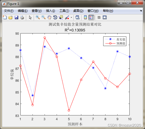
result = [T_test' T_sim' error']

%% V.  mapping 
figure
plot(1:N,T_test,'b:*',1:N,T_sim,'r-o')
legend(' True value ',' Predictive value ')
xlabel(' Prediction samples ')
ylabel(' Octane number ')
string = {
    ' Comparison of prediction results of octane number content in test set ';['R^2=' num2str(R2)]};
title(string)
toc

Click on “ function ”, The simulation results are as follows ：

result =

   88.5500   87.2278    0.0149
   84.7000   83.8908    0.0096
   88.8500   89.6147    0.0086
   88.2500   88.0039    0.0028
   88.7000   83.4154    0.0596
   87.9000   86.0295    0.0213
   87.0500   87.5730    0.0060
   85.3000   86.1662    0.0102
   88.4500   85.4190    0.0343
   88.0000   86.5528    0.0164

 Time has passed  2.260245  second .

Two . MATLAB Simulation II

%%%%%%%%%%%%%%%%%%%%%%%%%%%%%%%%%%%%%%%%%%%%%%%%%%%%
% function ：GRNN_PNN neural network 
% Environmental Science ：Win7,Matlab2015b
%Modi: C.S
% Time ：2022-06-27
%%%%%%%%%%%%%%%%%%%%%%%%%%%%%%%%%%%%%%%%%%%%%%%%%%%%

%% I.  Clear environment variables 
clear all
clc

tic
%% II.  Training set / Test set generation 
%%
% 1.  Import data 
load iris_data.mat

%%
% 2  Randomly generate training set and test set 
P_train = [];
T_train = [];
P_test = [];
T_test = [];
for i = 1:3
    temp_input = features((i-1)*50+1:i*50,:);
    temp_output = classes((i-1)*50+1:i*50,:);
    n = randperm(50);
    %  Training set ——120 Samples 
    P_train = [P_train temp_input(n(1:40),:)'];
    T_train = [T_train temp_output(n(1:40),:)'];
    %  Test set ——30 Samples 
    P_test = [P_test temp_input(n(41:50),:)'];
    T_test = [T_test temp_output(n(41:50),:)'];
end

%% III.  model  
result_grnn = [];
result_pnn = [];
time_grnn = [];
time_pnn = [];
for i = 1:4
    for j = i:4
        p_train = P_train(i:j,:);
        p_test = P_test(i:j,:);
       %% 
        % 1. GRNN Creation and simulation test 
        t = cputime;
        %  Creating networks 
        net_grnn = newgrnn(p_train,T_train);
        %  The simulation test 
        t_sim_grnn = sim(net_grnn,p_test);
        T_sim_grnn = round(t_sim_grnn);
        t = cputime - t;
        time_grnn = [time_grnn t];
        result_grnn = [result_grnn T_sim_grnn'];
       %%
        % 2. PNN Creation and simulation test 
        t = cputime;
        Tc_train = ind2vec(T_train);
        %  Creating networks 
        net_pnn = newpnn(p_train,Tc_train);
        %  The simulation test 
        Tc_test = ind2vec(T_test);
        t_sim_pnn = sim(net_pnn,p_test);
        T_sim_pnn = vec2ind(t_sim_pnn);
        t = cputime - t;
        time_pnn = [time_pnn t];
        result_pnn = [result_pnn T_sim_pnn'];
    end
end

%% IV.  Performance evaluation 
%%
% 1.  Accuracy rate accuracy
accuracy_grnn = [];
accuracy_pnn = [];
time = [];
for i = 1:10
    accuracy_1 = length(find(result_grnn(:,i) == T_test'))/length(T_test);
    accuracy_2 = length(find(result_pnn(:,i) == T_test'))/length(T_test);
    accuracy_grnn = [accuracy_grnn accuracy_1];
    accuracy_pnn = [accuracy_pnn accuracy_2];
end

%%
% 2.  Results contrast 
result = [T_test' result_grnn result_pnn];
accuracy = [accuracy_grnn;accuracy_pnn]
time = [time_grnn;time_pnn]

%% V.  mapping 
figure(1)
plot(1:30,T_test,'bo',1:30,result_grnn(:,4),'r-*',1:30,result_pnn(:,4),'k:^')
grid on
xlabel(' Test set sample number ')
ylabel(' Test set sample category ')
string = {
    ' Test set prediction results comparison (GRNN vs PNN)';[' Accuracy rate :' num2str(accuracy_grnn(4)*100) '%(GRNN) vs ' num2str(accuracy_pnn(4)*100) '%(PNN)']};
title(string)
legend(' True value ','GRNN Predictive value ','PNN Predictive value ')
figure(2)
plot(1:10,accuracy(1,:),'r-*',1:10,accuracy(2,:),'b:o')
grid on
xlabel(' Model number ')
ylabel(' Test set accuracy ')
title('10 Comparison of test set accuracy of models (GRNN vs PNN)')
legend('GRNN','PNN')
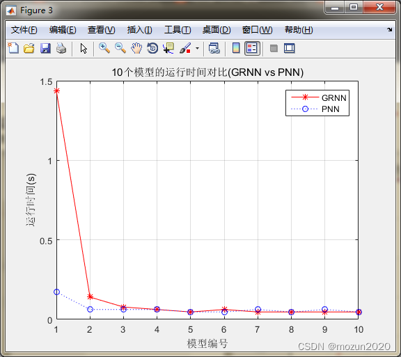
figure(3)
plot(1:10,time(1,:),'r-*',1:10,time(2,:),'b:o')
grid on
xlabel(' Model number ')
ylabel(' The elapsed time (s)')
title('10 Comparison of running time of models (GRNN vs PNN)')
legend('GRNN','PNN')
toc

Click on “ function ”, The simulation results are as follows ：

accuracy =

    0.3667    0.4000    1.0000    1.0000    0.3333    1.0000    1.0000    1.0000    1.0000    0.7000
    0.6333    0.7667    1.0000    1.0000    0.4667    0.9333    1.0000    1.0000    1.0000    0.9667


time =

    1.4352    0.1404    0.0780    0.0624    0.0468    0.0624    0.0468    0.0468    0.0468    0.0468
    0.1716    0.0624    0.0624    0.0624    0.0468    0.0468    0.0624    0.0468    0.0624    0.0468

 Time has passed  3.570447  second .

3、 ... and . Summary

RBF,GRNN,PNN, Example simulation of three neural networks for prediction analysis , In fact, in my own column 《MATLAB neural network 43 A case study 》 There are also three kinds of neural networks introduced in , Interested students can also move to the column , Link at the end of the article . Learn one every day MATLAB Little knowledge , Let's learn and make progress together ！

MATLAB neural network 43 A case study