Hierarchical clustering and case analysis

Hierarchical clustering

Hierarchical clustering (Hierarchical Clustering) It is a kind of clustering algorithm , A hierarchical nested clustering tree is created by calculating the similarity between different data points . In the cluster tree , Different categories of raw data points are the lowest level of the tree , The top layer of the tree is the root node of a cluster . There are two methods to create a cluster tree: bottom-up merging and top-down splitting .

As a human resources manager of a company , You can organize all employees into larger clusters , Such as supervisor 、 Managers and staff ; Then you can further divide it into smaller clusters , for example , Employee clusters can be further divided into sub clusters ： officer , General staff and interns . All these clusters form a hierarchy , It is easy to summarize or characterize data at all levels .

How to divide is appropriate ？

Intuitive to see , The data shown in the above figure is divided into 2 Clusters or 4 Each cluster is reasonable , even to the extent that , If the inside of each circle above contains a data set formed by a large amount of data , Then it may be divided into 16 Clusters are what you need .

On how many clusters a data set should be clustered into , It is usually a discussion about the scale at which we focus on this data set . One of the advantages of hierarchical clustering algorithm over partitioned clustering algorithm is that it can work on different scales （ level ） Show the clustering of the data set .

Hierarchical clustering algorithm （Hierarchical Clustering） It can be condensed （Agglomerative） Or split （Divisive）, Depending on the level of division is “ Bottom up ” still “ The top-down ”. 

Bottom up merging algorithm

The merging algorithm of hierarchical clustering calculates the similarity between two kinds of data points , Combine the two most similar data points among all data points , And iterate over and over again . To put it simply The merging algorithm of hierarchical clustering is to determine the similarity between data points of each category and all data points by calculating the distance between them , The smaller the distance , The higher the similarity . and Combine the two closest data points or categories , Generate a cluster tree .

The calculation of similarity

Hierarchical clustering uses Euclidean distance to calculate the distance between different categories of data points （ Similarity degree ）.

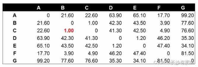
example ： The data points are as follows

                                              

  Calculate the Euclidean distance value respectively （ matrix ）

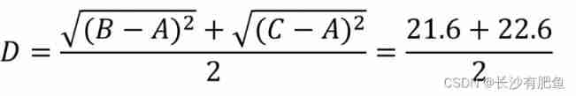
  take The data points B And data points C After the combination , Recalculate the distance matrix between data points of each category . The distance between data points is calculated in the same way as before . What needs to be explained here is the combination of data points (B,C) Calculation method with other data points . When we calculate (B,C) To A At a distance of , It needs to be calculated separately B To A and C To A Mean distance of .

After calculating data points D To the data point E Is the smallest of all distance values , by 1.20. This means that in all current data points （ Contains composite data points ）,D and E The most similar . So we put the data points D And data points E Are combined . And calculate the distance between other data points again .

The later work is to repeatedly calculate data points and data points , The distance between the data point and the combined data point . This step should be done by the program . Due to the small amount of data , We manually calculate and list the results of distance calculation and data point combination at each step .

The distance between two combined data points

There are three methods to calculate the distance between two combined data points , Respectively Single Linkage,Complete Linkage and Average Linkage. Before we start the calculation , Let's first introduce the three calculation methods and their advantages and disadvantages .

• Single Linkage： The method is to take the distance between the nearest two data points in the two combined data points as the distance between the two combined data points . This method is susceptible to extreme values . Two very similar composite data points may be combined because one of the extreme data points is close to each other .

• Complete Linkage：Complete Linkage The calculation method of is similar to that of Single Linkage contrary , The distance between the farthest two data points in the two combined data points is regarded as the distance between the two combined data points .Complete Linkage The problem with Single Linkage contrary , Two dissimilar composite data points may be unable to be combined due to the distance between their extreme values .

• Average Linkage：Average Linkage The calculation method of this method is to calculate the distance between each data point in two combined data points and all other data points . Take the mean of all distances as the distance between two composite data points . This method needs a lot of calculation , But the results are more reasonable than the first two .

We use Average Linkage Calculate the distance between combined data points . The following is the calculation of combined data points (A,F) To (B,C) Distance of , Here we calculate (A,F) and (B,C) The mean distance between two .

  Tree view

  Hierarchical clustering python

import pandas as pd

seeds_df = pd.read_csv('./datasets/seeds-less-rows.csv')
seeds_df.head()

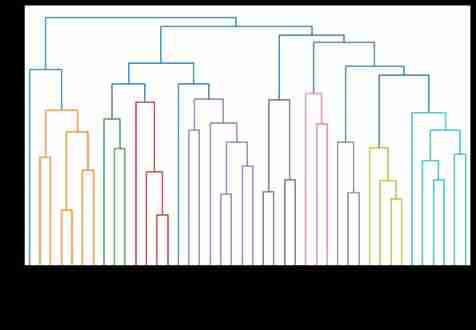
seeds_df.grain_variety.value_counts()  

Kama wheat        14
Rosa wheat        14
Canadian wheat    14
Name: grain_variety, dtype: int64

varieties = list(seeds_df.pop('grain_variety'))

samples = seeds_df.values

samples

array([[14.88  , 14.57  ,  0.8811,  5.554 ,  3.333 ,  1.018 ,  4.956 ],
       [14.69  , 14.49  ,  0.8799,  5.563 ,  3.259 ,  3.586 ,  5.219 ],
       [14.03  , 14.16  ,  0.8796,  5.438 ,  3.201 ,  1.717 ,  5.001 ],
       [13.99  , 13.83  ,  0.9183,  5.119 ,  3.383 ,  5.234 ,  4.781 ],
       [14.11  , 14.26  ,  0.8722,  5.52  ,  3.168 ,  2.688 ,  5.219 ],
       [13.02  , 13.76  ,  0.8641,  5.395 ,  3.026 ,  3.373 ,  4.825 ],
       [15.49  , 14.94  ,  0.8724,  5.757 ,  3.371 ,  3.412 ,  5.228 ],
       [16.2   , 15.27  ,  0.8734,  5.826 ,  3.464 ,  2.823 ,  5.527 ],
       [13.5   , 13.85  ,  0.8852,  5.351 ,  3.158 ,  2.249 ,  5.176 ],
       [15.36  , 14.76  ,  0.8861,  5.701 ,  3.393 ,  1.367 ,  5.132 ],
       [15.78  , 14.91  ,  0.8923,  5.674 ,  3.434 ,  5.593 ,  5.136 ],
       [14.46  , 14.35  ,  0.8818,  5.388 ,  3.377 ,  2.802 ,  5.044 ],
       [11.23  , 12.63  ,  0.884 ,  4.902 ,  2.879 ,  2.269 ,  4.703 ],
       [14.34  , 14.37  ,  0.8726,  5.63  ,  3.19  ,  1.313 ,  5.15  ],
       [16.84  , 15.67  ,  0.8623,  5.998 ,  3.484 ,  4.675 ,  5.877 ],
       [17.32  , 15.91  ,  0.8599,  6.064 ,  3.403 ,  3.824 ,  5.922 ],
       [18.72  , 16.19  ,  0.8977,  6.006 ,  3.857 ,  5.324 ,  5.879 ],
       [18.88  , 16.26  ,  0.8969,  6.084 ,  3.764 ,  1.649 ,  6.109 ],
       [18.76  , 16.2   ,  0.8984,  6.172 ,  3.796 ,  3.12  ,  6.053 ],
       [19.31  , 16.59  ,  0.8815,  6.341 ,  3.81  ,  3.477 ,  6.238 ],
       [17.99  , 15.86  ,  0.8992,  5.89  ,  3.694 ,  2.068 ,  5.837 ],
       [18.85  , 16.17  ,  0.9056,  6.152 ,  3.806 ,  2.843 ,  6.2   ],
       [19.38  , 16.72  ,  0.8716,  6.303 ,  3.791 ,  3.678 ,  5.965 ],
       [18.96  , 16.2   ,  0.9077,  6.051 ,  3.897 ,  4.334 ,  5.75  ],
       [18.14  , 16.12  ,  0.8772,  6.059 ,  3.563 ,  3.619 ,  6.011 ],
       [18.65  , 16.41  ,  0.8698,  6.285 ,  3.594 ,  4.391 ,  6.102 ],
       [18.94  , 16.32  ,  0.8942,  6.144 ,  3.825 ,  2.908 ,  5.949 ],
       [17.36  , 15.76  ,  0.8785,  6.145 ,  3.574 ,  3.526 ,  5.971 ],
       [13.32  , 13.94  ,  0.8613,  5.541 ,  3.073 ,  7.035 ,  5.44  ],
       [11.43  , 13.13  ,  0.8335,  5.176 ,  2.719 ,  2.221 ,  5.132 ],
       [12.01  , 13.52  ,  0.8249,  5.405 ,  2.776 ,  6.992 ,  5.27  ],
       [11.34  , 12.87  ,  0.8596,  5.053 ,  2.849 ,  3.347 ,  5.003 ],
       [12.02  , 13.33  ,  0.8503,  5.35  ,  2.81  ,  4.271 ,  5.308 ],
       [12.44  , 13.59  ,  0.8462,  5.319 ,  2.897 ,  4.924 ,  5.27  ],
       [11.55  , 13.1   ,  0.8455,  5.167 ,  2.845 ,  6.715 ,  4.956 ],
       [11.26  , 13.01  ,  0.8355,  5.186 ,  2.71  ,  5.335 ,  5.092 ],
       [12.46  , 13.41  ,  0.8706,  5.236 ,  3.017 ,  4.987 ,  5.147 ],
       [11.81  , 13.45  ,  0.8198,  5.413 ,  2.716 ,  4.898 ,  5.352 ],
       [11.27  , 12.86  ,  0.8563,  5.091 ,  2.804 ,  3.985 ,  5.001 ],
       [12.79  , 13.53  ,  0.8786,  5.224 ,  3.054 ,  5.483 ,  4.958 ],
       [12.67  , 13.32  ,  0.8977,  4.984 ,  3.135 ,  2.3   ,  4.745 ],
       [11.23  , 12.88  ,  0.8511,  5.14  ,  2.795 ,  4.325 ,  5.003 ]])

# Distance calculation linkage  And the tree view dendrogram
from scipy.cluster.hierarchy import linkage, dendrogram
import matplotlib.pyplot as plt

# Hierarchical clustering 
mergings = linkage(samples, method='complete')

# Tree view results 
fig = plt.figure(figsize=(10,6))
dendrogram(mergings,
           labels=varieties,
           leaf_rotation=90,
           leaf_font_size=6,
)
plt.show()

# Get the label result 
#maximum height Make it your own 
from scipy.cluster.hierarchy import fcluster
labels = fcluster(mergings, 6, criterion='distance')

df = pd.DataFrame({'labels': labels, 'varieties': varieties})
ct = pd.crosstab(df['labels'], df['varieties'])
ct

           

  The choice of different distances will produce different results

import pandas as pd

scores_df = pd.read_csv('./datasets/eurovision-2016-televoting.csv', index_col=0)
country_names = list(scores_df.index)
scores_df.head()

# Missing value fill , If you don't have one, you can count it by the full score 
scores_df = scores_df.fillna(12)

# normalization 
from sklearn.preprocessing import normalize
samples = normalize(scores_df.values)

samples

array([[0.09449112, 0.56694671, 0.        , ..., 0.        , 0.28347335,
        0.        ],
       [0.49319696, 0.        , 0.16439899, ..., 0.        , 0.41099747,
        0.        ],
       [0.        , 0.49319696, 0.12329924, ..., 0.        , 0.32879797,
        0.16439899],
       ...,
       [0.32879797, 0.20549873, 0.24659848, ..., 0.49319696, 0.28769823,
        0.        ],
       [0.28769823, 0.16439899, 0.        , ..., 0.        , 0.49319696,
        0.        ],
       [0.        , 0.24659848, 0.        , ..., 0.        , 0.20549873,
        0.49319696]])

from scipy.cluster.hierarchy import linkage, dendrogram
import matplotlib.pyplot as plt

mergings = linkage(samples, method='single')
fig = plt.figure(figsize=(10,6))
dendrogram(mergings,
           labels=country_names,
           leaf_rotation=90,
           leaf_font_size=6,
)
plt.show()

mergings = linkage(samples, method='complete')
fig = plt.figure(figsize=(10,6))
dendrogram(mergings,
           labels=country_names,
           leaf_rotation=90,
           leaf_font_size=6,
)
plt.show()