当前位置:网站首页>Several common optimization methods matlab principle and depth analysis
Several common optimization methods matlab principle and depth analysis
2022-07-03 13:29:00 【Haibao 7】
Catalog
There are various optimization problems in life or work , For example, every enterprise and individual should
A problem to consider “ At a certain cost , How to maximize profits ” etc. . The optimization method is a mathematical method , It is to study how to seek certain factors under given constraints ( The amount of ), To make a ( Or something ) The general name of some disciplines with optimal indicators . With the deepening of learning , Bloggers are increasingly discovering the importance of optimization methods , Most of the problems encountered in study and work can be modeled as an optimization model to solve , For example, the machine learning algorithm we are learning now , The essence of most machine learning algorithms is to build optimization models , Through the optimization method for the objective function ( Or loss function ) To optimize , To train the best model . The common optimization methods are gradient descent method 、 Newton method and quasi Newton method 、 Conjugate gradient method, etc .
1. Gradient descent method
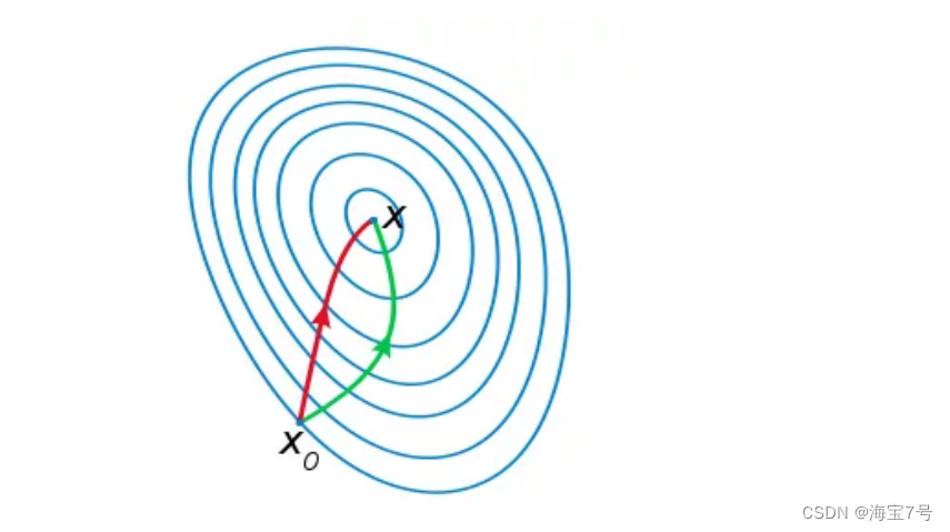
Gradient descent method is the earliest and simplest , It is also the most commonly used optimization method . Gradient descent method is easy to realize , When the objective function is convex , The solution of gradient descent method is the global solution . In general , The solution is not guaranteed to be the global optimal solution , The gradient descent method is not necessarily the fastest . The optimization idea of gradient descent method is to use the negative gradient direction of current position as the search direction , Because this direction is the fastest descent direction of the current position , So it's also called ” The steepest descent “. The steepest descent method is closer to the target value , The smaller the step , The slower forward . Search of gradient descent method
The schematic diagram of cable iteration is shown in the figure below :
The disadvantage of gradient descent method :
(1) Convergence slows down as we approach the minimum , As shown in the figure below ;
(2) There may be some problems in line search ;
(3) May be “ Zigzag ” Drop down .
The convergence speed of gradient descent method is obviously slower in the region close to the optimal solution , Using the gradient descent method to solve the problem requires many iterations .
In machine learning , Based on the basic gradient descent method, two gradient descent methods are developed , They are random gradient descent method and batch gradient descent method .
For a linear regression (Linear Logistics) Model , Suppose the following h(x) Is the function to fit ,J(theta) Is the loss function ,theta Is the parameter , The value to be solved iteratively ,theta It's solved , The function to be fitted in the end h(theta) It's coming out. . among m Is the number of samples in the training set ,n It's the number of features .
1.1 Batch gradient descent method (Batch Gradient Descent,BGD)
take J(theta) Yes theta Finding partial derivatives , Get each theta The corresponding gradient :

Because it is to minimize the risk function , So press each parameter theta Negative direction of gradient , To update each theta:

From the above formula, you can notice that , What it gets is a global optimal solution , But every iteration step , All the data in the training set , If m It's big , It is conceivable that the iteration speed of this method will be quite slow . therefore , This introduces another method —— Stochastic gradient descent .
For batch gradient descent method , Number of samples m,x by n Dimension vector , An iteration needs to put m All samples are brought into the calculation , One iteration, the amount of calculation is m*n^2.
1.2 Stochastic gradient descent (Stochastic Gradient Descent,SGD)
The risk function can be written as follows , The loss function corresponds to the gradient of each sample in the training set , The above batch gradient decline corresponds to all training samples :
Loss function for each sample , Yes theta Find the partial derivative to get the corresponding gradient , To update theta:

Random gradient descent is an iterative update of each sample , If the sample size is large ( For example, hundreds of thousands ), Then maybe only tens of thousands or thousands of samples , It's already theta Iteration to the optimal solution , Compared with the above batch gradient drop , More than 100000 training samples are needed for one iteration , One iteration cannot be optimal , If you iterate 10 Then we need to traverse the training samples 10 Time . however ,SGD One of the accompanying problems is that the noise is more BGD More , bring SGD It's not going to be optimization every time . Random gradient descent uses only one sample per iteration , One iteration, the amount of calculation is n^2, When the number of samples m Very big time , Random gradient descent iteration is much faster than batch gradient descent method . The relationship between the two can be understood in this way : The stochastic gradient descent method is at the cost of losing a small part of accuracy and increasing a certain number of iterations , In exchange for the improvement of overall optimization efficiency . The number of iterations increased is much less than the number of samples .
1.3 Summary
Batch gradient descent -– Minimize the loss function of all training samples , So that the final solution is the global optimal solution , That is, the parameter to be solved is to minimize the risk function , But it is inefficient for large-scale sample problems .
Stochastic gradient descent — Minimize the loss function for each sample , Although the loss function obtained in each iteration is not in the direction of global optimization , But the direction of the large whole is towards the global optimal solution , The final result is always near the global optimal solution , It is suitable for large-scale training samples .
2. Newton method and quasi Newton method
2.1 Newton method (Newton’s method)
Newton's iteration (Newton’s method) Also known as Newton - Ralph ( Raffson ) Method (Newton-Raphson method), It's Newton in 17 An approximate method for solving equations in real and complex fields was proposed in the 20th century . Newton method is a kind of approximate solution of equation in real number field and complex number field . Method to use the function f (x) To find the equation f (x) = 0 The root of the . The biggest characteristic of Newton's method is its fast convergence .
Have proved , If it's continuous , And the zero point to be solved is isolated , Then there is a region around zero , As long as the initial value is in this adjacent area , So Newton's method must converge . also , If not for 0, Then Newton's method will have the property of square convergence . Roughly speaking , That means every iteration , The effective number of Newton's results will be doubled .
Iteration method is also called toss method , It is the process of recursing a new value from the old value of a variable , The counterpart of the iterative method is the direct method ( Or it's called the first solution ), Solve the problem once and for all . Iterative algorithm is a basic method to solve problems by computer . It uses computers to calculate fast 、 Suitable for repetitive operation , Let the computer read a set of instructions ( Or a certain step ) repeat , At each execution of this set of instructions ( Or these steps ) when , Both derive a new value from the original value of the variable .

Use iterative algorithm to solve the problem , We need to do a good job in the following three aspects :
One 、 Determine the iteration variables
Among the problems that can be solved by iterative algorithm , There is at least one variable that can directly or indirectly continuously deduce new values from old values , This variable is the iteration variable .
Two 、 Establish an iterative relationship
The so-called iterative relation , It refers to how to deduce the formula of the next value from the previous value of a variable ( Or relationship ). The establishment of iterative relation is the key to solve the iterative problem , Usually you can use recursive or backward methods to complete .
3、 ... and 、 Control the iterative process
When does the iteration end ? This is the problem that must be considered when writing iterative programs . The iterative process cannot be carried out endlessly . The control of iterative process can be divided into two cases : One is that the number of iterations required is a certain value , It can be calculated ; The other is that the number of iterations required cannot be determined . In the former case , A fixed number of loops can be built to control the iterative process ; In the latter case , Further analysis is needed to arrive at the conditions that can be used to end the iterative process .
Geometrically , Newton's method is to use a quadric surface to fit the local surface where you are , and
Gradient descent method uses a plane to fit the current local surface , Usually , Quadric surfaces fit better than planar surfaces , Therefore, the descent path selected by Newton method will be more in line with the actual optimal descent path .
notes : The iterative path of red Newton method , Green is the iterative path of gradient descent method .
matlab Code :
 Defined function
function y=f(x)
y=f(x);% function f(x) The expression of
end
function z=h(x)
z=h(x);% function h(x) The expression of , function h(x) Is the function f(x) First derivative of
end
 The main program
x=X;% Initial value of iteration
i=0;% Iteration count
while i
x0=X-f(X)/h(X);% Newton iterative scheme
if abs(x0-X)>0.01;% Convergence judgment
X=x0;
else break
end
i=i+1;
end
fprintf('\n%s%.4f\t%s%d','X=',X,'i=',i) % Output results
Python The code shows the root of solving the equation with an example .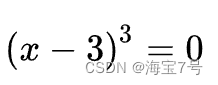
py file
def f(x):
    return (x-3)**3        ''' Definition  f(x) = (x-3)^3'''

def fd(x):
    return 3*((x-3)**2)    ''' Definition  f'(x) = 3*((x-3)^2)'''

def newtonMethod(n,assum):
    time = n
    x = assum
    Next = 0
    A = f(x)
    B = fd(x)
    print('A = ' + str(A) + ',B = ' + str(B) + ',time = ' + str(time))
    if f(x) == 0.0:
        return time,x
    else:
        Next = x - A/B
        print('Next x = '+ str(Next))
    if abs(A - f(Next)) < 1e-6:
        print('Meet f(x) = 0,x = ' + str(Next)) ''' Set the iteration jump out condition , At the same time, the output meets f(x) = 0 Of x value '''
    else:
        return newtonMethod(n+1,Next)

newtonMethod(0,4.0)    ''' Set from 0 Start counting ,x0 = 4.0'''
The advantages and disadvantages of Newton's method are summarized :
advantage : Second order convergence , Fast convergence ;
shortcoming : Newton's method is an iterative algorithm , Every step needs to solve the objective function Hessian The inverse of the matrix , The calculation is complicated .
2.2 Quasi Newton method (Quasi-Newton Methods)
Quasi Newton method is one of the most effective methods to solve nonlinear optimization problems , On 20 century 50 In the United States Argonne Physicists at the National Laboratory W.C.Davidon Put forward .Davidon The design of this algorithm at that time seemed to be one of the most creative inventions in the field of nonlinear optimization . Soon R. Fletcher and M. J. D. Powell It is proved that this new algorithm is much faster and more reliable than other methods , It makes the subject of nonlinear optimization advance by leaps and bounds overnight .
The essential idea of quasi Newton method Is to improve Newton's method every time you need to solve complex Hessian The defect of inverse matrix of matrix , It uses a positive definite matrix to approximate Hessian The matrix of the inverse , Thus, the complexity of operation is simplified . Like the steepest descent method, the quasi Newton method only requires that the gradient of the objective function be known at each iteration step .
Quasi Newton method and steepest descent method (Steepest Descent Methods) Just know the gradient of the objective function at each iteration . By measuring the change in gradient , A model of objective function is constructed to produce superlinear convergence . This method is much better than the steepest descent method , Especially for difficult problems .
in addition , Because the quasi Newton method does not need the information of the second derivative , So sometimes it's better than Newton's method (Newton’s Method) More effective . Now , The optimization software contains a lot of quasi Newton algorithm to solve unconstrained , constraint , And large scale optimization problems .
Quasi Newton method is one of the most effective methods in solving nonlinear equations and optimization calculation , It is a kind of Newton type iterative method that makes the calculation amount of each iteration less and maintains superlinear convergence .
By measuring the change in gradient , A model of objective function is constructed to produce superlinear convergence . This method is much better than the steepest descent method , Especially for difficult problems . in addition , Because the quasi Newton method does not need the information of the second derivative , So sometimes it's more efficient than Newton's method . Now , The optimization software contains a lot of quasi Newton algorithm to solve unconstrained , constraint , And large scale optimization problems .
The basic idea of quasi Newton method is as follows . First, construct a quadratic model of the objective function in the current iteration parameters :

here Bk It's a symmetric positive definite matrix , So we take the optimal solution of the quadratic model as the search direction , And get a new iteration point :

Among them, we require step size ak Satisfy Wolfe Conditions . This iteration is similar to Newton's method , The difference is to use approximate Hesse matrix Bk Substitute for real Hesse matrix . So the key point of quasi Newton method is the matrix in each iteration step Bk Update . Now suppose you get a new iteration xk+1, And a new quadratic model is obtained :
Use the information in the previous step as much as possible to select Bk. In particular

It is also the secant equation . The commonly used quasi Newton method is DFP Algorithm and BFGS Algorithm , Details can be searched by yourself .
3. conjugate gradient method (Conjugate Gradient)
Conjugate gradient method is a method between steepest descent method and Newton method , It just uses the first derivative information , But it overcomes the shortcoming of the steepest descent method , It also avoids the need of storage and calculation of Newton method Hesse The disadvantage of matrix inversion , Conjugate gradient method is not only one of the most useful methods to solve large-scale linear equations , It is also one of the most effective algorithms for large-scale nonlinear optimization . In all kinds of optimization algorithms , Conjugate gradient method is very important . Its advantage is that it needs less storage , It has step convergence , High stability , And it doesn't need any foreign parameters .
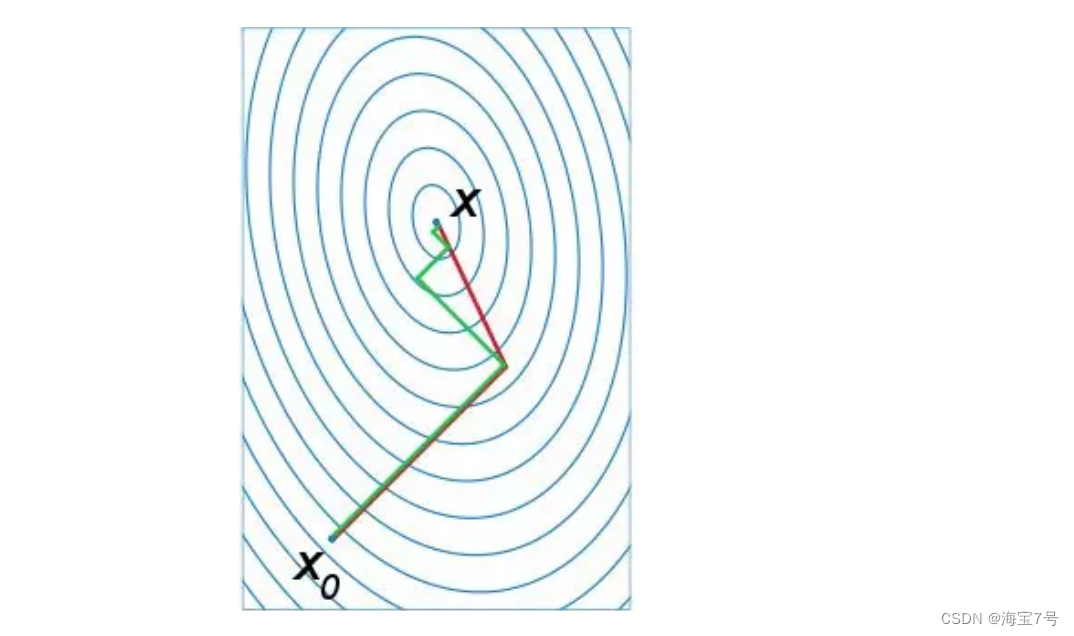
The following figure is the path comparison diagram of conjugate gradient method and gradient descent method for searching the optimal solution , notes : Green is gradient descent , Red for conjugate gradient method
matlab Code :
function [x] = conjgrad(A,b,x)
r=b-A*x;
p=r;
rsold=r'*r;
for i=1:length(b)
Ap=A*p;
alpha=rsold/(p'*Ap);
x=x+alpha*p;
r=r-alpha*Ap;
rsnew=r'*r;
if sqrt(rsnew)<1e-10 break;
end
p=r+(rsnew/rsold)*p;
rsold=rsnew;
end
end
conjugate gradient method (Conjugate Gradient)
Each of its search directions is conjugate , And these search directions d It's just a combination of the negative gradient direction and the search direction of the previous iteration , therefore , Less storage , Convenient calculation .
advantage : Small amount of storage required , It has step convergence , High stability , And it doesn't need any foreign parameters . It can be used for unconstrained convex quadratic programming problems , Save storage space .
shortcoming : Convergent dependence K matrix .
Suggest : It's not a large-scale operation, so you don't need to use .
For more information, please refer to numerical analysis 、 Optimization courses and books .
The steepest descent and conjugate gradient methods are used to solve a linear equation
%% linear equation Ax=b
A = [4,-2,-1;-2,4,-2;-1,-2,3];
b = [0;-2;3];
The steepest descent
%%  The steepest descent
x0 = [0;0;0];
iter_max = 1000;
for i = 1:iter_max
    r = A*x0 - b;
    alpha = (r'*r)/(r'*A*r);
    x = x0 - alpha*r;
    if norm(x-x0)<=10^(-8)
        break
    end
    x0 = x;
end
conjugate gradient method
```csharp
%%  conjugate gradient method
x0 = [0;0;0];
r0 = A*x0 - b;
p0 = -r0;
iter_max = 1000;
for i = 1:iter_max
    alpha = (r0'*r0)/(p0'*A*p0);
    x = x0 + alpha*p0;
    r = r0 + alpha*A*p0;
    beta = (r'*r)/(r0'*r0);
    p = -r + beta*p0;
    if norm(x-x0)<=10^(-8)
        break
    end
    x0 = x;
    r0 = r;
    p0 = p;
end
4. Heuristic optimization method
Heuristic algorithm (heuristic algorithm) It is relative to the optimization algorithm . At this stage , The heuristic algorithm is mainly based on the natural body algorithm , There are mainly ant colony algorithm 、 Simulated annealing 、 Neural network and so on .
Various specific implementation methods of modern heuristic algorithms are relatively independent , There are certain differences between them . historically , Modern heuristic algorithms mainly include : Simulated annealing algorithm (SA)、 Genetic algorithm (ga) (GA)、 List search algorithm (ST)、 Evolutionary programming (EP)、 Evolutionary strategy (ES)、 Ant colony algorithm (ACA)、 Artificial neural network (ANN). If we consider the different coding schemes of decision variables , There can be fixed length codes ( Static coding ) And variable length encoding ( Dynamic coding ) Two kinds of schemes .
For details, please refer to Baidu Encyclopedia or Wikipedia , Or the blog of relevant experts .
边栏推荐
- Idea full text search shortcut ctr+shift+f failure problem
- 【电脑插入U盘或者内存卡显示无法格式化FAT32如何解决】
- Red hat satellite 6: better management of servers and clouds
- 8皇后问题
- 今日睡眠质量记录77分
- Start signing up CCF C ³- [email protected] chianxin: Perspective of Russian Ukrainian cyber war - Security confrontation and sanctions g
- My creation anniversary: the fifth anniversary
- Internet of things completion -- (stm32f407 connects to cloud platform detection data)
- Sword finger offer 16 Integer power of numeric value
- AI scores 81 in high scores. Netizens: AI model can't avoid "internal examination"!
猜你喜欢
Flink SQL knows why (XV): changed the source code and realized a batch lookup join (with source code attached)
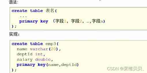
MySQL constraints

Seven habits of highly effective people
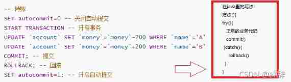
MySQL
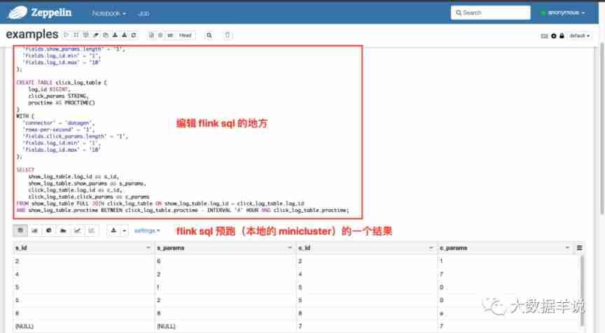
Flink SQL knows why (17): Zeppelin, a sharp tool for developing Flink SQL

【历史上的今天】7 月 3 日:人体工程学标准法案;消费电子领域先驱诞生;育碧发布 Uplay
Solve system has not been booted with SYSTEMd as init system (PID 1) Can‘t operate.

人身变声器的原理
![[colab] [7 methods of using external data]](/img/cf/07236c2887c781580e6f402f68608a.png)
[colab] [7 methods of using external data]
[today in history] July 3: ergonomic standards act; The birth of pioneers in the field of consumer electronics; Ubisoft releases uplay
随机推荐
The reasons why there are so many programming languages in programming internal skills
Start signing up CCF C ³- [email protected] chianxin: Perspective of Russian Ukrainian cyber war - Security confrontation and sanctions g
MapReduce implements matrix multiplication - implementation code
DQL basic query
Error handling when adding files to SVN:.... \conf\svnserve conf:12: Option expected
Logback 日志框架
February 14, 2022, incluxdb survey - mind map
[Database Principle and Application Tutorial (4th Edition | wechat Edition) Chen Zhibo] [Chapter 6 exercises]
Flick SQL knows why (10): everyone uses accumulate window to calculate cumulative indicators
JSON serialization case summary
When updating mysql, the condition is a query
Servlet
Reptile
Kivy教程之 如何通过字符串方式载入kv文件设计界面(教程含源码)
[Database Principle and Application Tutorial (4th Edition | wechat Edition) Chen Zhibo] [Chapter IV exercises]
用户和组命令练习
JS 将伪数组转换成数组
今日睡眠质量记录77分
Sword finger offer 16 Integer power of numeric value
[Database Principle and Application Tutorial (4th Edition | wechat Edition) Chen Zhibo] [sqlserver2012 comprehensive exercise]